Hyperbolic PDEs
Convergence and Consistency
A convergent scheme is one where the numerical solution (as computed by the scheme) approximates the analytical solution to the PDE and that the approximation improves as the spatial and temporal spacings tend towards zero, (h, k)\to0.
Stability
Consistency is not the only property required to ensure a scheme converges. If a scheme is truly convergent, then as v_m^n converges to u(t, x), then this means v_m^n is bounded. For any given scheme, we may draw a stability region \Lambda that restricts the possible values of h and k that guarantee stability. A stability region is a bounded and nonempty region in the first quadrant of \mathbb R^2. The origin (0, 0) must be included in \Lambda as it serves as the accumulation point for (h, k). What this means is for a sequence of (h_i, i_i) pairs, each successive pair must converge to (0, 0) as i\to\infty.
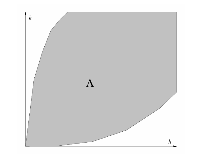
A finite difference scheme P_{k, h}v_m^n=0 for a 1st order equation is stable in its stability region \Lambda if there is an integer J such that for any time T>0, there is a constant C_T such that
h\sum\limits_{m=-\infty}^{\infty}\left|v_m^n\right|^2\leq C_Th\sum\limits_{j=0}^J\sum\limits_{m=-\infty}^{\infty}\left|v_m^j\right|^2 \tag{1}
for 0\leq nk\leq T and (k, h)\in\Lambda.
Before explaining the meaning behind Eq. 1, we first review some useful notation. For any grid function w, the quantity \lVert w\rVert_h is the L_2 norm of w and is a measure of the size of the solution. For most applications, the L_2 norm gives the magnitude or physical significance of something (e.g., L_2 norm of the velocity vector is the velocity magnitude).
\lVert w\rVert_h=\sqrt{h\sum\limits_{m=-\infty}^{\infty}\left|w_m\right|^2} \tag{2}
Using Eq. 2, Eq. 1 can be rewritten as
\lVert v^n\rVert_h\leq\sqrt{C_T\sum\limits_{j=0}^J\lVert v^j\rVert_h^2}\leq C_T^*\sum\limits_{j=0}^J\lVert v^j\rVert_h \tag{3}
where C_T^* is an arbitrary constant. The central idea behind Eq. 1 and Eq. 3 is that there is an upper bound in the amount of growth that can occur for a solution at time 0\leq t\leq T. This bound is at most a constant multiple of the sum of the solution norms, \lVert v^j\rVert_h of the first J+1 steps. In general, J=0 for single-step schemes, as well as some multi-step schemes.
A sufficient condition for the FTFS scheme can be derived by considering a general form of the scheme with coefficients \alpha and \beta.
v_m^{n+1}=\alpha v_m^n+\beta v_{m+1}^n
Substituting into Eq. 3, we get
\begin{aligned} \sum\limits_{m=-\infty}^{\infty}\left|v_m^{n+1}\right|^2 & =\sum\limits_{m=-\infty}^{\infty}\left|\alpha v_m^n+\beta v_{m+1}^n\right|^2 \\ & \leq\sum\limits_{m=-\infty}^{\infty}\left(|\alpha|^2\left|v_m^n\right|^2+2|\alpha||\beta|\left|v_m^n\right|\left|v_{m+1}^n\right|+|\beta|^2\left|v_{m+1}^n\right|^2\right) \\ & \leq\sum\limits_{m=-\infty}^{\infty}\left[|\alpha|^2\left|v_m^n\right|^2+|\alpha||\beta|\left(\left|v_m^n\right|^2+\left|v_{m+1}^n\right|^2\right)+|\beta|^2\left|v_{m+1}^n\right|^2\right] \end{aligned}
The last inequality comes from the fact that (x-y)^2\geq0 so 2xy\leq x^2+y^2. The last summation may be split into a sum across m indices and m+1 indices. Since -\infty<m<\infty, we may re-index the m+1 summation without affecting the sequence. This is akin to replacing all instances of m in the sum with m-1. Doing so gives
\begin{aligned} \sum\limits_{m=-\infty}^{\infty}\left|v_m^{n+1}\right|^2 & \leq\sum\limits_{m=-\infty}^{\infty}\left(|\alpha|^2\left|v_m^n\right|^2+|\alpha||\beta|\left|v_m^n\right|^2\right)+\sum\limits_{m=-\infty}^{\infty}\left(|\alpha||\beta|\left|v_{m+1}^n\right|^2+|\beta|^2\left|v_{m+1}^n\right|^2\right) \\ & =\sum\limits_{m=-\infty}^{\infty}\left(|\alpha|^2\left|v_m^n\right|^2+|\alpha||\beta|\left|v_m^n\right|^2+|\alpha||\beta|\left|v_m^n\right|^2+|\beta|^2\left|v_m^n\right|^2\right) \\ & =\left(|\alpha|+|\beta|\right)^2\sum\limits_{m=-\infty}^{\infty}\left|v_m^n\right|^2 \end{aligned}
To recap, we have shown that Eq. 3 becomes
\sum\limits_{m=-\infty}^{\infty}\left|v_m^{n+1}\right|^2\leq(|\alpha|+|\beta|)^2\sum\limits_{m=-\infty}^{\infty}\left|v_m^n\right|^2=(|\alpha|+|\beta|)^{2n}\sum\limits_{m=-\infty}^{\infty}\left|v_m^0\right|^2
For the last equation, we have gone back n temporal grid levels to the initial condition. If the coefficient |\alpha|+|\beta|\leq1, then the scheme will be stable. With the case of FTFS, \alpha=1+a\lambda and \beta=a\lambda. Substituting gives
|1+a\lambda|+|a\lambda|\leq1
Therefore, -1\leq a\lambda\leq0 is a necessary condition for stability for FTFS.
Stability for finite difference schemes is closely related to the concept of well-posedness for IVPs for PDEs. For the definition below, we require that these schemes are 1st order differentiation with respect to time.
The initial value problem for the 1st order PDE Pu=0 is well-posed if there exists a constant C_T such that any solution u(t, x) satisfies
\int\limits_{-\infty}^{\infty}\left|u(t, x)\right|^2\,\mathrm dx\leq C_T\int\limits_{-\infty}^{\infty}\left|u(0, x)\right|^2\,\mathrm dx \tag{4}
for 0\leq t\leq T and T\geq0.
The Lax-Richtmyer Equivalence Theorem
A finite difference scheme for a PDE whose initial value problem is well-posed is convergent if and only if the scheme is both consistent and stable.
The equivalence theorem ties together the concept of consistency and stability for determining whether a finite difference scheme converges. Previously, we focused on the idea that consistency and stability imply convergence. Another consequence of the theorem is the reverse direction; that is, all unstable or inconsistent schemes will never be convergent.
The CFL Condition
A necessary condition for stability for many explicit schemes that follow the form of the wave equation is |a\lambda|\leq1 where \lambda=\frac kh. This condition is called the Courant-Friedrichs-Lewy (CFL) condition.
For an explicit scheme for an equation of the form
v_m^{n+1}=\alpha v_{m-1}^n+\beta v_m^n+\gamma v_{m+1}^n \tag{5}
where \lambda=\frac kh is held constant, a necessary condition for stability is the requirement that |a\lambda|\leq1. For the case of systems of equations, where \textbf v is a vector and \boldsymbol{\alpha}, \boldsymbol{\beta}, and \boldsymbol{\gamma} are matrices, the CFL condition becomes |a_i\lambda|\leq1 for all eigenvalues a_i of the matrix \textbf A.
We first consider the case of a single equation and then extend it to a system. If we assume that |a\lambda|>1, then if we consider the point (t, x)=(1, 0), we see that the solution to the PDE depends on the values of u_0(x) at x=-a by following the characteristic curve connecting (t, x)=(1, 0) to the x axis.

A similar argument can be used to show that there is no explicit, consistent scheme for the hyperbolic PDE that is stable for all values of \lambda. In other words, there will always exist a \lambda where the scheme is unstable as (h, k)\to(0, 0).
Conceptually, the CFL condition relates the numerical speed of propagation with the speed of propagation of the PDE. We may rewrite Eq. 5 as
\frac 1{\lambda}\leq|a|
where \frac 1{\lambda}=\frac hk is the numerical speed of propagation for the scheme. This speed must always exceed the PDE’s speed of propagation in order for the scheme to converge. If the numerical scheme cannot propagate the solution as fast as the PDE’s solution, then the solution of the scheme cannot possibly converge to the solution of the PDE.