Flows Through Miniature Flow Passages
Size Classification
There is no universal classification for “miniature” in miniature flow passages, but the most popular one is
\begin{aligned} D_H & =10-100\mathrm{\,\mu m} & \mathrm{microchannels} \\ D_H & =100\mathrm{\,\mu m}-1\mathrm{\,mm} & \mathrm{minichannels} \\ D_H & =1-3\mathrm{\,mm} & \mathrm{macrochannels} \\ D_H & >6\mathrm{\,mm} & \mathrm{conventional} \end{aligned}
And for heat exchangers
\begin{aligned} D_H & =1-100\mathrm{\,\mu m} & \text{microheat exchangers} \\ D_H & =100\mathrm{\,\mu m}-1\mathrm{\,mm} & \text{mesoheat exchangers} \\ D_H & =1-6\mathrm{\,mm} & \text{compact heat exchangers} \\ D_H & >6\mathrm{\,mm} & \text{conventional} \end{aligned}
Classical fluid mechanics makes the continuum assumption, where fluids may be treated as homogeneous and continuous. For miniature flow passages, this assumption may begin to break down at the smallest D_H length scales. For a fluid to be treated as a continuum, there must be
Sufficient molecules such that the flow is molecularly chaotic. This is typically satisfied when there are \sim100 molecules across the smallest dimension of the flow passage and is typically not the limiting condition governing the applicability of the continuum assumption.
More frequent molecule-molecule interactions than molecule-wall interactions. The molecular behavior must be dominated by random, molecular collisions between molecules rather than with the solid boundaries.
Condition 2 is more likely to be violated for small flow passages as the intermolecular distance becomes a non-negligible quantity when compared to the flow passage dimension. When molecular-wall interactions reach the same order of magnitude as molecular interaction, the continuum assumption partially breaks down. And when molecule-wall dominates over molecular interaction, the continuum is no longer valid.
The continuum approximation is more likely to break down for gases than it is for liquids. Recall that the molecular mean free path \lambda_{\mathrm{mol}} is the average distance a molecule will travel before colliding with another molecule. For gases, this equation may be written in terms of the specific gas constant R.
\lambda_{\mathrm{mol}}=\nu\sqrt{\frac {\pi}{2RT}} \tag{1}
The Knudsen number compares \lambda_{\mathrm{mol}} to a length scale of the flow passage, l_c.
\mathrm{Kn}_{l_c}=\frac {\lambda_{\mathrm{mol}}}{l_c} \tag{2}
For continuum to be valid, \mathrm{Kn}_{l_c}\ll1. For liquids, intermolecular distances are much smaller than in gases, roughly \sim1 nm. Therefore, continuum is less likely to break down since each molecule is in a constant state of collision with its neighbor. The key effect to consider for liquid flows in this case is the effect of surface forces near the boundaries. These effects are negligible in conventional, large scale flow passages since the surface area-to-volume ratio is small. But as the passage size decreases, this ratio increases, and liquid-surface force effects are no longer negligible. When this is the case, continuum mechanics may still be applied, but must be modified to include these surface effects.
Regimes in Gas-Carrying Vessels
Slip Flow and Temperature Jump Regime
This flow regime occurs when the gas flow is rarified and may occur if the channel is sufficiently small. The distinguishing features for this flow regime compared to the flow of rarified gas through a larger channel are
Viscous forces become more dominant due to the larger surface area-to-volume ratios present in small microchannels.
Large density variations may occur across the microchannel, augmented by pressure and temperature variations down the channel. For adiabatic and moderately-heated channel flows, variations in pressure are a significant driving force behind large density variations.
Axial heat conduction down the length of the channel is non-negligible due to the small volumes present in microchannels. While for larger channels, axial heat conduction could be neglected if \mathrm{Pe}_{D_H}\gtrsim100, this is not the case for applications with microchannels. Neglecting axial heat conduction in theoretical analysis may lead to significant error when compared to experimental data.
Conventional fluid mechanics assumes no-slip boundary conditions and thermal equilibrium at the wall for viscous fluids. This is not necessarily the case for flows of rarified gases
The conventional no-slip and thermal equilibrium assumption at the wall boundaries is not necessarily true for rarified flows. This is because conventional fluid mechanics assumes the gas and the wall are at interfacial equilibrium at large scales. This assumption begins to break down as we approach the field of rarified flows.
In conventional fluid mechanics, we assume that gas molecules colliding with the wall exchange their momentum and energy with the wall’s molecules, and that when leaving the wall, the molecule’s momentum and energy (and therefore, temperature) are statistically adjusted to match that of the wall’s molecules. This kind of reasoning holds for large scale flows since gas molecules collide more frequently with each other than with the wall. The intermolecular path for these flows is so small relative to the length scale of the flow passage that they, statistically speaking, are more likely to hit another molecule upon leaving the wall rather than the other wall boundary of the flow passage. This is what is meant by the condition \mathrm{Kn}\ll1.
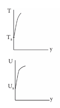
The case is different for flows in microchannels, where the collision rate is now much lower on account of the intermolecular path, \lambda_{\mathrm{mol}}, being close to the same order of magnitude as the characteristic passage length. Gas molecules in this case do not collide with each other frequently enough near the wall to fully equilibrate with the wall before moving back into the core flow. Because the wall and gas immediately next to each other do not share the same velocity and temperature, the wall and gas are in nonequilibrium and we have
\begin{aligned} u_g\neq U_s \\ T_g\neq T_s \end{aligned}
The subscripts s and g mean the property is applied to the wall surface or gas respectively. When this occurs, there is a velocity slip and temperature jump at the boundaries.
Let the wall surface velocity and temperature be U_s and T_s respectively. Under slip and thermal nonequilibrium conditions, the fluid-side boundary conditions will be a corrected U_s^* and T_s^* property that is related to the actual wall U_s and T_s boundary values. This is done by assuming that at some distance g normal to the wall, the velocity and temperature are constant and equal to the corrected values mentioned.
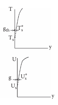
The distance from the wall for both velocity and thermal boundaries is approximated using the kinetic theory of gases.
\begin{aligned} g_{\mathrm{th}} & \approx\frac {2-\alpha_{\mathrm{th}}}{\alpha_{\mathrm{th}}}\frac {2\gamma}{\gamma+1}\frac {\lambda_{\mathrm{mol}}}{\mathrm{Pr}} \\ g & \approx\frac {2-\alpha}{\alpha}\lambda_{\mathrm{mol}} \end{aligned} \tag{3}
where \alpha is the tangential momentum accommodation coefficient (or specular reflection coefficient) and \alpha_{\mathrm{th}} is the thermal energy accommodation coefficient. The corrected fluid-side interface velocity is
U_s^*-U_s=\frac {2-\alpha}{\alpha}\lambda_{\mathrm{mol}}\left(\frac {\partial u}{\partial y}\right)_{y=0}+\frac 34\frac {\mu}{\rho T_s}\left(\frac {\partial T}{\partial x}\right)_{y=0}-C_1\lambda_{\mathrm{mol}}^2\left[\frac {\partial^2u}{\partial y^2}+\frac 12\frac {\partial^2u}{\partial x^2}+\frac 12\frac {\partial^2u}{\partial z^2}\right]_{y=0} \tag{4}
The corrected fluid-side interface temperature is
T_s^*-T_s=\frac {2-\alpha_{\mathrm{th}}}{\alpha_{\mathrm{th}}}\frac {2\gamma}{\gamma+1}\frac {\lambda_{\mathrm{mol}}}{\mathrm{Pr}}\left(\frac {\partial T}{\partial y}\right)_{y=0}-C_2\lambda_{\mathrm{mol}}^2\left[\frac {\partial^2T}{\partial y^2}+\frac 12\frac {\partial^2T}{\partial x^2}+\frac 12\frac {\partial^2T}{\partial z^2}\right]_{y=0} \tag{5}
The coefficients C_1 and C_2 may be calculated using
\begin{aligned} C_1 & =\frac 98 \\ C_2 & =\frac 9{128}\frac {177\gamma-145}{\gamma+1} \end{aligned}
The second term in Eq. 4 is referred to as thermal creep. In most cases, where the flow is moderately rarified, the second-order terms can be neglected. This results in the following simplifications for U_s^* and T_s^*.
\begin{aligned} U_s^*-U_s & =\frac {2-\alpha}{\alpha}\lambda_{\mathrm{mol}}\left(\frac {\partial u}{\partial y}\right)_{y=0}+3\sqrt{\frac {R_uT}{8\pi}}\frac {\lambda_{\mathrm{mol}}}T\left(\frac {\partial T}{\partial s}\right)_{y=0} \\ T_s^*-T_s & =\frac {2-\alpha_{\mathrm{th}}}{\alpha_{\mathrm{th}}}\frac {2\gamma}{\gamma+1}\frac {\lambda_{\mathrm{mol}}}{\mathrm{Pr}}\left(\frac {\partial T}{\partial y}\right)_{y=0} \end{aligned} \tag{6}
The subscript s denotes the fluid motion path and \left(\partial T/\partial y\right)_{y=0} is the tangential gas temperature gradient at the wall. Let \Omega and E be the momentum and energy fluxes associated with the gas molecules. Furthermore, let \mathrm{in} denote incident, \mathrm{refl} denote reflected, and s denote reflected for gas molecules that have reached equilibrium with the wall. We may express the accommodation coefficients in terms of their momentum and energy fluxes as
\begin{aligned} \alpha & =\frac {\Omega_{\mathrm{refl}}-\Omega_{\mathrm{in}}}{\Omega_s-\Omega_{\mathrm{in}}} \\ \alpha_{\mathrm{th}} & =\frac {E_{\mathrm{refl}}-E_{\mathrm{in}}}{E_s-E_{\mathrm{in}}} \end{aligned} \tag{7}
These definitions for \alpha and \alpha_{\mathrm{th}} aren’t the most useful in a practical sense. Using Eq. 7, they must be determined experimentally. However, for most gases and solid boundaries, their accommodation coefficients are close to one: \alpha=\alpha_{\mathrm{th}}\approx1. Song and Yovanovich (1987) proposed an empirical correlation for \alpha_{\mathrm{th}} for metallic surfaces where 273\leq T_s\leq1250 K.
\alpha_{\mathrm{th}}=F\frac {M_G}{6.8+M_G}+(1-F)\frac {2.4\xi}{(1+\xi)^2} \tag{8}
where
\begin{aligned} \xi & =\frac {M_G}{M_{\mathrm{solid}}} \\ F & =\exp\left[-0.57\left(\frac {T_s}{273}-1\right)\right] \end{aligned}
For nearly all applications, g\ll l_c and g_{\mathrm{th}}\ll l_c so the boundary conditions for slip conditions and thermal nonequilibrium at the wall surface are
\begin{aligned} U(0) & =U_s^* \\ T(0) & =T_s^* \end{aligned}
We can shorten Eq. 6 by substituting
\begin{aligned} \beta_v & =\frac {2-\alpha}{\alpha} \\ \beta_T & =\frac {2-\alpha_{\mathrm{th}}}{\alpha_{\mathrm{th}}}\frac {2\gamma}{\gamma+1}\frac 1{\mathrm{Pr}} \end{aligned} \tag{9}
Therefore, Eq. 6 becomes
\begin{aligned} U_s^*-U_s & =\beta_v\lambda_{\mathrm{mol}}\left(\frac {\partial u}{\partial y}\right)_s+3\sqrt{\frac {R_uT}{8\pi}}\frac {\lambda_{\mathrm{mol}}}T\left(\frac {\partial T}{\partial s}\right)_s \\ T_s^*-T_s & =\beta_T\lambda_{\mathrm{mol}}\left(\frac {\partial T}{\partial y}\right)_s \end{aligned}
The slip flow regime is nearly always laminar and as such, analytical solutions are possible for many different geometries and boundary conditions.
Slip Couette Flow
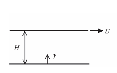
The Couette flow model derived in Chapter 4. Internal Laminar Flow assumed no velocity slip and temperature jump. This is only valid when \mathrm{Ma}\mathrm{Kn}_{l_c}\ll1 as all streamwise derivative terms are negligible except pressure gradient. For consistency, use the following definitions for the Couette flow model, where the top surface is moving with velocity U.
Apply the same reduction as shown in , the momentum and energy equations reduce down to
\begin{gathered} \frac {\partial^2u}{\partial y^2}=0 \\ k\frac {\partial^2T}{\partial y^2}+\mu\left(\frac {\partial u}{\partial y}\right)^2=0 \end{gathered} \tag{10}
The boundary conditions at the bottom and top plates are
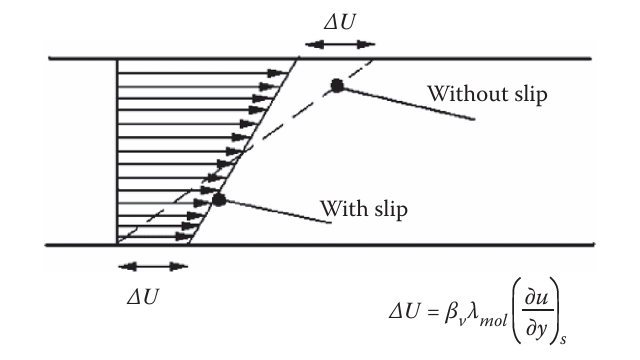
\begin{aligned} u(0) & =\beta_v\lambda_{\mathrm{mol}}\frac {\partial u}{\partial y} \\ u(H) & =U-\beta_v\lambda_{\mathrm{mol}}\frac {\partial u}{\partial y} \end{aligned} \tag{11}
The hydrodynamic solution (momentum equation) with the boundary conditions applied is
\frac uU=\frac 1{1+2\beta_v\mathrm{Kn}_H}\left(\frac yH+\beta_v\mathrm{Nu}_H\right) \tag{12}
The Knudsen number uses the channel height as the characteristic length, \mathrm{Kn}_H=\lambda_{\mathrm{mol}}/H. The profile for u(y) is still linear, but the slope is larger when compared to the no-slip condition.
The volumetric flow rate per unit depth is determined by integrating u(y) from y=0 to y=H. The result of Q=\frac 12HU is identical to the no-slip flow rate for conventional channels. The Fanning friction factor, or skin friction coefficient, for the bottom plate is
C_f=\frac {\tau_0}{\frac 12\rho U^2}=\frac 2{\mathrm{Re}_H\left(1+2\beta_v\mathrm{Kn}_H\right)}=\frac 2{\mathrm{Re}_H+2\sqrt{\frac {\pi\gamma}2}\beta_v\mathrm{Ma}} \tag{13}
where \tau_0=\mu\left(\mathrm du/\mathrm dy\right)_{y=0} is the shear stress at the bottom plate and \mathrm{Re}_H=UH/\nu. If we define the Poiseuille number as \mathrm{Po}=C_f\mathrm{Re}_{D_H}=2C_f\mathrm{Re}_H, then the ratios between the slip and no-slip Poiseuille numbers become
\frac {\mathrm{Po}_{\mathrm{slip}}}{\mathrm{Po}_{\mathrm{no-slip}}}=\frac 1{1+2\beta_v\mathrm{Kn}_H}=\frac 1{1+2\beta_v\sqrt{\frac {\pi\gamma}2}\frac {\mathrm{Ma}}{\mathrm{Re}_H}} \tag{14}
The Poiseuille number ratio is a measure of how the skin friction coefficient changes between the slip and no-slip conditions (\mathrm{Re}_H is constant between the two cases). As a result, Eq. 14 shows that velocity slip reduces the wall friction.
Now, use Fig. 2 (b) to calculate the heat transfer coefficient. If we assume the bottom plate is adiabatic and the top plate experiences a heat flux along the outer surface, then the boundary conditions become
\begin{gathered} \left.\frac {\mathrm dT}{\mathrm dy}\right|_{y=0}=0 \\ \left.-k\frac {\mathrm dT}{\mathrm dy}\right|_{y=H}=h_0(T-T_{\infty}) \end{gathered}
Differentiating Eq. 12 and substituting into the energy equation in Eq. 10, we get
T=-\frac 12\varphi y^2+\frac {kH\varphi}{h_0}+\frac {H^2\varphi}2+\beta_T\mathrm{Kn}_HH^2\varphi+T_{\infty} \tag{15}
where \varphi=\mu\Phi/k is a parameter that is related to the viscous dissipation.