Part B: The Acoustic Wave Equation
Derivation of the Wave Equation
Notation
The instantaneous density is defined as \rho=\rho(\mathbf r, t). For a given medium, the density may vary or fluctuate across position and time. Though there may be small fluctuations present, \rho will generally vary across a steady, averaged value in the medium called the equilibrium ambient density \rho_0=\rho_0(\mathbf r). The equilibrium ambient density may be a function of position (e.g., density of air varies as height above sea level increases), but is not time-dependent. We may define condensation as the density difference relative to \rho_0. Mathematically, this is defined as
s=\frac {\rho(\mathbf r, t)-\rho_0(\mathbf r)}{\rho_0(\mathbf r)} \tag{1}
In a similar vein to density, we may define instantaneous and ambient equilibrium pressures as \mathcal P=\mathcal P(\mathbf r, t) and \mathcal P_0=\mathcal P_0(\mathbf r) respectively. The degree of pressure fluctuation between the instantaneous pressure and equilibrium pressure is the acoustic (or sound) pressure.
p(\mathbf r, t)=\mathcal P(\mathbf r, t)-\mathcal P_0(\mathbf r) \tag{2}
Lastly, temperature is denoted by T_K. The subscript K signifies the units must be in Kelvin. In acoustics, we generally do not consider significant timescales where the temperature changes drastically or instantly. Therefore, we make no distinction between instantaneous and equilibrium ambient temperature.
The Lossless Acoustic Wave Equation
We apply three principles when deriving the lossless wave equation. The term “lossless” in this case refers to the lack of viscous effects in the fluid that the wave is propagating through.
Newton’s 2nd Law
Conservation of Mass (Continuity)
Medium Equation of State
Newton’s 2nd Law
For small perturbations, where |p|\ll\mathcal P_0, we have the following relation called the linearized Euler equation. The derivation comes from a simplification of the Navier-Stokes equation. The derivation will not be given here.
\frac {\partial\mathbf u}{\partial t}+\frac 1{\rho_0}\nabla\mathbf p=\mathbf 0 \tag{3}
where \nabla\mathbf p is the gradient of the acoustic pressure.
Conservation of Mass
Since mass is always conserved in an acoustic field, we also have the continuity equation.
\frac {\partial\rho}{\partial t}+\rho_0\nabla\cdot\mathbf u=0 \tag{4}
Equation of State
For a thermally perfect gas, we have the following state relation.
\mathcal P=\rho RT_K \tag{5}
There is also an adiabatic state equation related to the adiabatic process p\propto \rho^{\gamma} where \gamma is the specific heat ratio. For diatomic gases and air, \gamma=1.4.
\frac {\mathcal P}{\mathcal P_0}=\left(\frac {\rho}{\rho_0}\right)^{\gamma} \tag{6}
In general, we may apply a 1st order Taylor series approximation to \mathcal P(\rho) centered on \mathcal P_0=\mathcal P(\rho_0) to get
p=\mathcal P(\rho)-\mathcal P(\rho_0)\approx\left.\frac {\partial\mathcal P}{\partial\rho}\right|_{\rho_0}(\rho-\rho_0)=\left.\frac {\partial\mathcal P}{\partial\rho}\right|_{\rho_0}\rho_0s
where s is the condensation, defined above. Define the coefficient of s as the adiabatic bulk modulus
\mathcal B=\rho_0\left.\frac {\partial\mathcal P}{\partial\rho}\right|_{\rho_0} \tag{7}
The adiabatic bulk modulus can be thought of as the volumetric stiffness of the fluid.
Therefore, the acoustic pressure is simply
p=\mathcal Bs=\mathcal B\frac {\rho-\rho_0}{\rho_0} \tag{8}
Derivation from Conservation Laws
From Eq. 8, we may differentiate with respect to time to get \frac {\partial p}{\partial t}=\mathcal B\frac {\partial s}{\partial t}. Additionally, from the definition of s, we also have \frac {\partial s}{\partial t}=\rho_0\frac {\partial\rho}{\partial t}. Assembling everything together gives
\frac 1{\mathcal B}\frac {\partial p}{\partial t}+\nabla\cdot\mathbf u=0
Next, we may eliminiate the \nabla\cdot\mathbf u by taking the divergence of Eq. 3 and substituting the \nabla\cdot\mathbf u above to get
-\frac 1{\mathcal B}\frac {\partial^2\rho}{\partial t^2}+\frac 1{\rho_0}\nabla^2p=0
Further simplification by relating \mathcal B with the speed of sound, c=\sqrt{\mathcal B/\rho_0}, gives the 3D classical acoustic wave.
\boxed{\nabla^2p=\frac 1{c^2}\frac {\partial^2\rho}{\partial t^2}} \tag{9}
Speed of Sound Relations
We have the following relation for speed of sound from its thermodynamic definition.
\boxed{c=\sqrt{\frac {\gamma\mathcal P_0}{\rho_0}}=\sqrt{\gamma RT_K}} \tag{10}
where \mathcal P_0 and \rho_0 are the ambient pressure and density respectively. To prove Eq. 10, differentiate Eq. 5 with respect to \rho and substitute into c=\sqrt{\left.\frac {\partial\mathcal P}{\partial\rho}\right|_{\mathrm{ad}}}.
The relation derived above in Eq. 10 is only valid for gases that obey Eq. 5. For other substances like solids or liquids, Eq. 10 cannot be used. Generally, c is measured and used to relate to other quantities. In general though, c depends on T_K and composition (c in freshwater is different than that in saltwater).
Traveling Wave Solutions
Helmholtz Equation
From Eq. 9, we assume that the wave is harmonic so p(\mathbf r,t) is a sinuisoidal function with respect to time. This allows us to relate the pressure as
\underline p(\mathbf r,t)=\underline{\underline p}(\mathbf r)e^{j\omega t} \tag{11}
Note that the coefficient \underline{\underline p} is double-underlined to signify that it refers to the amplitude of the complex-valued pressure function \underline p. Substituting Eq. 11 into Eq. 9 gives the Helmholtz equation.
\nabla^2\underline{\underline p}+k^2\underline{\underline p}(\mathbf r)=0 \tag{12}
where k=\frac {\omega}c is called the acoustic wavenumber with units of \mathrm L^{-1}.
Harmonic Plane Waves
For a plane wave, we make the simplification that the wave only propagates in the x direction. Therefore
\underline{\underline p}(\mathbf r)=\underline{\underline p}(x, y, z)=\underline{\underline p}(x)
Moreover, since \underline{\underline p} no longer depends on y and z, then \nabla^2\underline{\underline p} reduces to the second derivative of \underline{\underline p}. Therefore, Eq. 12 reduces down to an ODE.
\frac {\partial^2\underline{\underline p}}{\partial x^2}+k^2\underline{\underline p}=0 \tag{13}
The solution to Eq. 13 is given by \underline{\underline p}(x)=\underline A\exp(-jkx)+\underline B\exp(jkx). Therefore Eq. 11 for a harmonic plane wave becomes
\boxed{\underline p(x, t)=\underline Ae^{j(\omega t-kx)}+\underline Be^{j(\omega t+kx)}} \tag{14}
The first term, \underline A\exp[j(\omega t-kx)] represents a wave propagating in the +x direction. Similarly, the second term, \underline B\exp[j(\omega t+kx)] represents a wave propagating in the -x direction.
Particle Velocity
Before proceeding, we should explicitly cover the distinction between two velocity quantities for any given acoustic wave problem. The speed of sound, denoted by c, is the velocity at which a pressure disturbance (or acoustic wave) will propagate through a medium.
The particle velocity, denoted by \mathbf u, indicates how quickly an individual particle oscillates in an acoustic wave. If the wave is harmonic, then \mathbf u will also be harmonic. Therefore, each particle will sinusoidally oscillate by a very small amount. For the case of a harmonic plane wave, each particle will oscillate in the x direction by u=|\mathbf u| amount.
For air at standard pressure and temperature, c\simeq340 \mathrm{m/s}. However, u is generally on the order of magnitude of 1-10^6 \mathrm{\mu m/s}. Broadly speaking, u\ll c and is multiple orders of magnitude smaller.
To compute the particle velocity, we solve the linearized Euler equation, Eq. 3, for \underline{\mathbf u}. In the case of a 1D harmonic plane wave, then \underline{\mathbf u}=\underline u\hat x and \nabla\underline p=\frac {\partial\underline p}{\partial x}\hat x. Therefore, Eq. 3 becomes
\frac {\partial u}{\partial t}=-\frac 1{\rho_0}\frac {\partial p}{\partial x}
Next, we must make an assumptions about the wave itself. Assume the propagation direction is specified and is in the x direction with amplitude \underline A. The complete expression in Eq. 14 now reduces down to \underline p(x, t)=\underline A\exp\left[j(\omega t-kx)\right]. Furthermore, since the wave is harmonic, we know that the particle velocity vector must also be harmonic. Assume that the particle velocity in the x-direction is given by
\underline u=\underline Ue^{j(\omega t-kx)} \tag{15}
Substitute this form into the simplified Euler equation above and solve for the amplitude \underline U.
\underline U=\frac {\underline A}{\rho_0c} \tag{16}
This is the magnitude of the particle velocity. We may then derive the complete particle velocity vector for a harmonic plane wave as
\boxed{\underline{\mathbf u}=\underline u_{\pm}(x, t)\hat x=\pm\frac {\underline p(x, t)}{\rho_0c}\hat x} \tag{17}
The \pm notation indicates the direction of wave propagation. If the wave is propagating in the -x direction, we would take the negative branch of Eq. 17 to obtain that wave’s particle velocity vector.
If we assume a harmonic wave is comprised of two independent harmonic plane waves traveling in opposite directions, then the governing pressure equation is
\underline p(x, t)=\underline Ae^{j(\omega t-kx)}+\underline Be^{j(\omega t+kx)}\equiv\underline p_+(x, t)+\underline p_-(x, t)
The particle velocity for this is then
\underline u(x, t)=\frac {\underline p_+(x, t)}{\rho_0c}-\frac {\underline p_-(x, t)}{\rho_0c}=\frac {\underline Ae^{j(\omega t-kx)}}{\rho_0c}-\frac {\underline Be^{j(\omega t+kx)}}{\rho_0c}
Note that \underline u(x, t)\neq\frac {\underline p(x, t)}{\rho_0c}. For waves comprised of multiple waves, the particle velocity must be derived by summing up the particle velocities for each individual wave.
The expression for \underline{\mathbf u} in Eq. 17 is noticeably complex. To determine the real particle velocity that would be physically observed, take the real part of Eq. 17.
\boxed{\mathbf u=\pm\frac {\left|A\right|}{\rho_0c}\cos(\omega t-kx+\theta_A)\hat x} \tag{18}
In most cases, we are more interested in the amplitude of the particle oscillation, rather than the full periodic motion. That is not to say the phase angle of Eq. 18 is unimportant. Therefore, take the magnitude of Eq. 18 to determine the particle speed. For a plane wave, the physical particle velocity in the x-direction is
u(x)=\frac {\left|A\right|}{\rho_0c}
Particle Displacement
Since \bm{\xi}=\frac {\mathrm d\mathbf u}{\mathrm dt}, we may integrate with respect to time and assume the starting point is the origin. For the case of a harmonic plane wave propagating in the x direction, only \xi_x will be nonzero.
\bm{\xi}=\frac {\underline p(x, t)}{j\rho_0c\omega}\hat x \tag{19}
Phase Angle
The complex amplitude, \underline A for a wave propagating in the x direction in Eq. 14, can be decomposed into a magnitude term and phase angle term.
\underline A=\left|\underline A\right|e^{j\theta_A}
The phase angle accounts for any offset in the wave. The complex pressure in Eq. 14 now becomes
\underline p(x, t)=\left|\underline A\right|e^{j(\omega t-kx+\theta_A)} \tag{20}
The real pressure that is physically observed is simply the real part of Eq. 20.
p(x, t)=\mathrm{Re}\left[\underline p(x, t)\right]=\left|\underline A\right|\cos(\omega t-kx+\theta_A) \tag{21}
The real pressure in a plane wave, Eq. 21, also reveals the role \omega and k play in constructing the acoustic field. The term \omega is the angular frequency and has units of \mathrm{rad/s}. It is related to the wave’s frequency by
f=\frac {\omega}{2\pi} \tag{22}
where f has units of \mathrm{Hz}. The wave’s frequency represents the number of wave cycles repeated per second. The frequency is directly used to calculate the temporal period of the wave, which is the length of time each wave cycle takes.
T=\frac 1f=\frac {2\pi}{\omega} \tag{23}
Note that the period here describes a period in time. There is also a spatial period, called the wavelength, \lambda. This is the physical distance the wave covers before it repeats itself.
\lambda=\frac {2\pi}k \tag{24}
The k in Eq. 24 is the wavenumber and is the spatial analog of the angular frequency. The units of k are \mathrm{rad/m}, similar to how \omega has units of \mathrm{rad/s}.
k=\frac {\omega}c \tag{25}
We may relate the wavelength to the period directly by substituting Eq. 25 into Eq. 24 and using Eq. 22.
\lambda=cT=\frac cf \tag{26}
Propagation in Arbitrary Direction
The previous examples assumed the wave propagated in the same direction as the abscissa. For cases where the wave propagates in an arbitrary direction with respect to the x axis, our quantities for k and x now become a vector. Without loss of generality, assume the wave propagates at an angle \theta with respect to the x axis. Now, the equation for the pressure field becomes the dot product of the wavenumber vector and position vector.
\underline p(\mathbf r, t)=\underline Ae^{j(\omega t-\mathbf k\cdot\mathbf r)} \tag{27}
The position vector is defined as \mathbf r=x\hat x+y\hat y+z\hat z. The wavenumber vector is defined similarly as
\mathbf k=k_x\hat x+k_y\hat y+k_z\hat z
We have, by the magnitude, that \lVert\mathbf k\rVert^2=k_x^2+k_y^2+k_z^2. Each component of \mathbf k can be computed based off the overall magnitude \lVert\mathbf k\rVert=\frac {\omega}c. For instance, in the 2D case, we have
\begin{aligned} k_x & =\lVert\mathbf k\rVert\cos\theta=\frac {\omega}c\cos\theta \\ k_y & =\lVert\mathbf k\rVert\sin\theta=\frac {\omega}c\sin\theta \end{aligned}
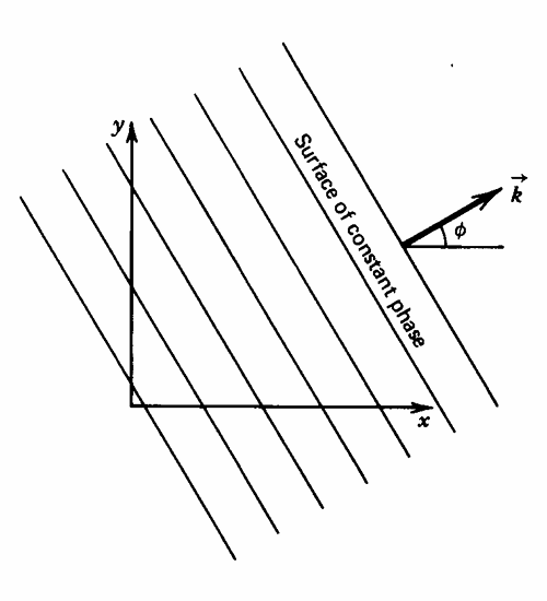
A natural question to ask is how the pressure field in Eq. 27 describes a plane wave propagating through space. Inspecting the form of Eq. 27, for a given amplitude \left|\underline A\right|, the pressure is constant when the exponential is constant. Rewriting \underline A in polar form, we have
\underline p(\mathbb r, t)=\left|\underline A\right|e^{j(\omega t-\mathbf k\cdot\mathbf r+\theta_A)}=\left|\underline A\right|e^{j\phi}
where \phi is the phase. When \phi is constant, then the pressure is constant. If we assume a 2D wave propagating in the xy plane, then \phi can be written as
y=-\frac {k_x}{k_y}x-\frac {C-\omega t-\theta_A}{k_y}
The last term is constant along a line of constant \phi. This describes a series of lines with slope -\frac {k_x}{k_y} that is perpendicular to \mathbf k. Since these lines (surfaces in 3D) of constant pressure are perpendicular to the propagation direction, the wave structure described is a plane wave.
Harmonic Spherical Waves
The other type of wave that can be created is the spherical wave. Unlike a plane wave, spherical waves propagate in all directions simultaneously from a point source. With these wave types, the surface of constant pressure becomes a sphere in 3D or circle in 2D centered on the source.
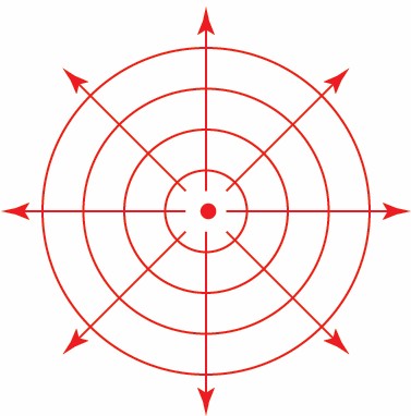
To derive \underline p(\mathbf r, t), we must solve Eq. 12 in spherical coordinates. Recall that in spherical coordinates, we have (x, y, z)\mapsto(r, \theta, \varphi) where r is the distance to the origin, \theta is the azimuth angle, and \varphi is the zenith angle with respect to the z axis. However, by symmetry, we may drop the dependence of \underline p(\mathbf r, t) on \theta and \varphi, leaving \underline p=\underline p(r, t). The Laplacian in spherical coordinates with \theta and \varphi dependence eliminated is
\nabla^2\underline p=\frac {\partial^2\underline p}{\partial r^2}+\frac 2r\frac {\partial\underline p}{\partial r}=\frac 1r\frac {\partial^2}{\partial r^2}\left[r\underline p(r, t)\right]
Expanding the Laplacian in Eq. 12, we get
\frac 1r\frac {\partial^2}{\partial r^2}\left[r\underline p(r, t)\right]+k^2\underline p(r, t)=0
We may assume a harmonic spherical wave of the form \underline p(r, t)=\underline{\underline p}(r)e^{j\omega t}. Substituting, we may eliminate the exponential, leaving behind
\frac {\partial^2}{\partial r^2}\left[r\underline{\underline p}(r)\right]+k^2r\underline{\underline p}(r)=0
This is identical to the ODE derived for the plane wave but transformed with r\underline{\underline p}(r) instead. Therefore, we may re-use the solution Eq. 14 with r\underline{\underline p} instead. Normalizing both sides by r to isolate \underline{\underline p} gives
\underline{\underline p}(r)=\frac {\underline A}re^{-jkx}+\frac {\underline B}re^{jkx} \tag{28}
The first term represents a spherical wave propagating outwards radially and the second represents one propagating in the opposite direction towards the source. Spherical waves that propagate away from the source are called diverging waves whereas those that propagate inwards are called converging waves. Depending on the boundary conditions, \underline A=0 or \underline B=0 to recover a single spherical wave propagating inwards or outwards in Eq. 28.
Let’s assume the wave under consideration is a diverging wave. Expressing \underline A in polar form, the acoustic pressure that is physically observed is
p(r, t)=\frac {\left|\underline A\right|}re^{j(\omega t-kr+\theta_A)} \tag{29}
Note that the pressure term in Eq. 29 is \propto\frac 1r. As the wave travels farther and farther away from its source, r increases resulting in p(r, t) decreasing. The cause of this is the increase in surface area of the imaginary sphere encompassing the wave. Since the surface area increases and energy is conserved, the wave amplitude must therefore decrease. This phenomenon is called spherical spreading and exists despite ignoring viscous effects. That is, the pressure amplitude decrease is not due to energy dissipation as the governing equation in Eq. 12 is lossless.
Spherical spreading generally dominates in most cases, especially “near” the source. Sound may not sound very loud close by due to energy conservation spreading across the increased surface area as the wave propagates from its source. Energy dissipation plays a minor to almost-negligible role in this.
Particle Velocity
Since we assume the spherical wave is harmonic, then Eq. 3 becomes
\frac {\partial\underline{\mathbf u}}{\partial t}+\frac 1{\rho_0}\nabla\underline p=j\omega\underline{\mathbf u}+\frac {\partial\underline p}{\partial r}\hat r=0
From this, we can see that the particle velocity \underline{\mathbf u} only has a \hat r direction. The pressure derivative term can be evaluated by differentiating Eq. 28 with respect to r. For a diverging wave, \underline B=0.
\frac {\partial\underline p}{\partial t}=\frac {\underline A}re^{j(\omega t-kr)}\left(-\frac 1r-jk\right)
Substituting and solving for \underline{\mathbf u}, then
\boxed{\underline{\mathbf u}=\left(1-\frac j{kr}\right)\frac {\underline p(r, t)}{\rho_0c}\hat r} \tag{30}
Particle Displacement
Like Eq. 19, integrate Eq. 30 with respect to time.
\boxed{\bm{\underline \xi}=\left(1-\frac j{kr}\right)\frac {\underline p(r, t)}{j\rho_0c\omega}\hat r} \tag{31}
Specific Acoustic Impedance
Like mechanical impedance, which is defined as the ratio between a force and velocity quantity, specific acoustic impedance describes the level of resistance that occurs when an acoustic pressure is applied to an arbitrary system.
\underline z=\frac {\underline p}{\underline{\mathbf u}\cdot\hat n_{\mathrm{in}}} \tag{32}
where \underline{\mathbf u} is the particle velocity vector and \hat n_{\mathrm{in}} is the unit vecotr in the direction of wave propagation. For a plane wave, \hat n_{\mathrm{in}}=\hat x so
\boxed{\underline z=\rho_0c\equiv z_0} \tag{33}
The term z_0 can be calculated from the fluid’s ambient density and speed of sound, two intrinsic properties to the fluid. Since this property is a function of two fluid properties, z_0 is also a property of a fluid. We call z_0 the characteristic impedance.
For a spherical wave, \hat n_{\mathrm{in}}=\hat r so \underline z becomes
\boxed{\underline z=\frac {\rho_0c}{1-\frac j{kr}}} \tag{34}
From Eq. 34, we can see that \underline z\neq z_0 clearly as \underline z=\underline z(kr). But if kr\gg1, then \underline z\to z_0 for spherical waves. This condition only occurs if the radial distance r dominates the wavenumber and is therefore, only valid in the farfield. From Eq. 24, we may rewrite this condition to be in terms of \lambda, which is a more-easily recognized property of the wave.
r\gg\frac {\lambda}{2\pi}
Derived Acoustic Quantities
Acoustic Intensity
The instantaneous acoustic intensity is related to the flow of power per unit area in the wave. It is defined as
\mathbf I_i(t)=p(t)\mathbf u(t) \tag{35}
Both quantities, p(t) and \mathbf u(t), must be real. The time-averaged acoustic intensity is determined by averaging \mathbf I_i(t) across a period, where we assume T\gg\frac {2\pi}{\omega}.
\mathbf I(t)=\frac 1T\int_0^T\mathbf I_i(t)\,\mathrm dt \tag{36}
Plane Wave
We have the following for p(x, t) and \mathbf u(x, t) for harmonic plane waves.
\begin{aligned} p(x, t) & =A\cos(\omega t-kx) \\ \mathbf u(x, t) & =\frac A{\rho_0c}\cos(\omega t-kx)\hat x \end{aligned}
By Eq. 35, we have
\boxed{\mathbf I_i(t)=\frac {A^2}{\rho_0c}\cos^2(\omega t-kx)\hat x} \tag{37}
By the double angle formula, express the \cos^2(\omega t-kx) in terms of \cos\left[2(\omega t-kx)\right]. Taking the integral, the cosine term disappears so all we’re left with is
\boxed{\mathbf I=\frac {A^2}{2\rho_0c}\hat x} \tag{38}
Spherical Wave
The time-average acoustic intensity is
\boxed{\mathbf I=\frac {A^2}{2r^2\rho_0c}} \tag{39}
Effective Pressure
Also known as the root mean square (RMS) pressure, it is determined by taking the square root of the time-average of p^2(t).
P_e=\sqrt{\frac 1T\int_0^Tp^2(t)\,\mathrm dt} \tag{40}
For a harmonic plane wave, where p(x, t)=A\cos(\omega t-kx), the effective pressure is
\boxed{P_e=\frac {\left|\underline A\right|}{\sqrt 2}} \tag{41}
Using Eq. 38, the acoustic intensity is also
\boxed{\mathbf I=\frac {P_e^2}{\rho_0c}\hat x} \tag{42}
For a spherical wave, p(r, t)=\frac Ar\cos(\omega t-kr) so
\boxed{P_e=\frac {\left|\underline A\right|}{r\sqrt 2}} \tag{43}
Using Eq. 39, the acoustic intensity is also
\boxed{\mathbf I=\frac {P_e^2(r)}{\rho_0c}\hat r} \tag{44}
Both formulas for \mathbf I for spherical and plane waves follow the same general form.
\mathbf I=\frac {P_e^2}{\rho_0c}\hat n_{\mathrm{in}}
where \hat n_{\mathrm{in}} is the unit vector in the direction of wave propagation and P_e is the effective pressure. For plane and spherical waves, \hat n_{\mathrm{in}}=\hat x or \hat r and P_e=\frac A{\sqrt 2} or \frac A{r\sqrt2} respectively.
Power
The total power for an acoustic wave is the integral of Eq. 36 across the entire surface \mathcal S.
\Pi=\int\limits_{\mathcal S}\mathbf I\cdot\mathbf n_s\,\mathrm dS \tag{45}
Plane Wave
From Eq. 38, \mathbf I is constant for a given x position. Therefore, Eq. 45 becomes
\Pi=\frac {S|\underline A|^2}{2\rho_0c} \tag{46}
where S is the cross-sectional area of the plane wave.
Spherical Wave
From Eq. 44, at a given radius R from the source, the radial acoustic intensity is constant since P_e(R) is constant and so is \rho_0c. Therefore, we have
\boxed{\Pi(R)=\frac {4\pi R^2}{\rho_0c}P_e^2(R)} \tag{47}
For spherical waves, recall that the governing form of Eq. 12 assumed no dissipation or loss of energy to the surroundings. Additionally, for all space excluding the point source, there is no additional source of energy for the wave. Therefore, by conservation of energy, we must have that \Pi(R_1)=\Pi(R_2) where R_1<R_2. This same line of reasoning can be made to deduce that \Pi(x_1)=\Pi(x_2) for plane waves, where x_1<x_2.
Acoustic Energy Density
Defined as the instantaneous energy per unit volume, the acoustic energy density may be calculated by summing both the kinetic and potential energy of the wave.
\varepsilon_i(t)=\frac 12\rho_0u^2(t)+\frac 12\left(\frac {p(t)}{\rho_0c}\right)^2 \tag{48}
The total energy E(t) is determined by integrating \varepsilon_i(t) across the entire volume \mathcal V.
E(t)=\int\limits_{\mathcal V}\varepsilon_i(t)\,\mathrm dV \tag{49}
Both u(t) and p(t) must be the real quantities in Eq. 48. Similar to Eq. 36, we may define a time-averaged energy density as
\varepsilon=\frac 1T\int_0^T\varepsilon_i(t)\,\mathrm dt \tag{50}
Plane Wave
For a plane wave, we have from Eq. 50
\varepsilon=\frac {P_e^2(x)}{\rho_0c^2} \tag{51}
Spherical Wave
For a spherical wave, we have from Eq. 50
\varepsilon=\frac {P_e^2(r)}{\rho_0c^2}\left(1+\frac 1{2k^2r^2}\right) \tag{52}
The Decibel Scale
Humans can perceive sounds ranging from acoustic pressures of 20 \mathrm{\mu Pa} to 2 \mathrm{Pa}. This is a 10^5 order of magnitude difference. Moreover, since energy is proportional to P_e^2, this range drastically increases from an energy perspective. We introduce a logarithmic scale to accommodate the large range in acoustic pressures.
Sound Intensity Level
The most widely used logarithmic scale for describing sound level is the decibel scale. The intensity level of an acoustic intensity \mathbf I is defined by
\mathrm{IL}=10\log_{10}\left(\frac {\lVert\mathbf I\rVert}{I_{\mathrm{ref}}}\right) \tag{53}
The reference intensity, I_{\mathrm{ref}}, is defined as the acoustic intensity at the lowest sound intensity perceivable by humans. Generally, I_{\mathrm{ref}}=10^{-12} \mathrm{W/m^2}.
Sound Pressure Level
The sound pressure level is similar in form to Eq. 53.
\mathrm{SPL}=20\log_{10}\left(\frac {P_e}{P_{\mathrm{ref}}}\right) \tag{54}
The reference pressure is usually taken to be 20 \mu\mathrm{Pa}. This value is somewhat arbitrary, but was deemed reference as it is the hearing threshold for a 1 \mathrm{kHz} acoustic wave. By the properties of logarithm, every time the sound pressure is increased by a factor of 10, 20 \mathrm{dB} is added to \mathrm{SPL}.
Humans can generally hear from 0 \mathrm{dB} to 100 \mathrm{dB}.
Problem: Compute the peak-to-peak displacement of a plane wave with \mathrm{SPL}=100 \mathrm{dB} at 500 \mathrm{kHz}.
Solution: From Eq. 54, solve for P_e.
P_e=P_{\mathrm{ref}}\cdot 10^5=2\times10^{-5}\times10^5=2\space\mathrm{Pa}
Relate the effective pressure to the acoustic pressure using Eq. 41. Note that \underline A in this case represents the pressure amplitude.
\underline A=P_e\sqrt2
Next, compute the particle velocity vector \underline{\mathbf u} using
\underline{\mathbf u}=\frac {\underline A}{\rho_0c}\hat x=\frac {P_e\sqrt2}{\rho_0c}\hat x
The magnitude of \underline{\mathbf u} is simply \frac {P_e\sqrt2}{\rho_0c}. To relate to peak-to-peak displacement, make use that \bm{\xi} is harmonic.
\underline{\mathbf u}=\frac {\mathrm d\underline{\bm{\xi}}}{\mathrm dt}=j\omega\underline{\bm{\xi}}
Take the magnitude of both sides and the j disappears.
\left|\underline{\bm{\xi}}\right|=\frac {P_e\sqrt2}{\rho_0\omega c}=\frac {P_e\sqrt2}{2\pi\rho_0fc}
The frequency is known. We assume the sound wave is propagating through air, so \rho_0=1.184 \mathrm{kg/m^3} and c=344 \mathrm{m/s}.