Classical Thermodynamics for Compressible Substances
Introduction and Definitions
Thermodynamics is the study of energy and matter. That is, how energy and matter change throughout a process. Broadly speaking, we may list four laws or postulates from empirical evidence.
The Zeroth Law of Thermodynamics
Bodies are in thermal equilibrium with each other only when they have the same degree of “hotness”. In modern physics, we use temperature to describe “hotness” between objects. So two objects with the same temperature are in thermal equilibrium.
The First Law of Thermodynamics
Energy cannot be created nor destroyed, it is conserved. One of the key conclusions from this law is that perpetual motion machines cannot exist.
The Second Law of Thermodynamics
Entropy can only be created, it cannot be destroyed. Therefore, it is impossible to reverse any natural process in its entirety and there is a “time dependence” in all processes that arises from the inability to destroy entropy.
The State Postulate
The number of independent thermodynamic properties needed to define a state can be determined prior.
When analyzing an object or region, we typically classify objects or regions as systems or surroundings. A thermodynamic system is simply a finite portion of matter or restricted portion of space upon which we are interested in. For example, when considering a volume of air inside a piston, we may declare the enclosed air to be our system. The surroundings on the other hand is anything not enclosed by the system. For the example above, the piston, outer environment, etc. make up the surroundings. Sometimes, environment is also used to describe the surroundings. The system is enclosed by the control surface. This is a surface, typically imaginary but can also be real, that separates the system from its surroundings. Oftentimes, it is helpful to classify the system based off the object or region it is enclosing. The system is called a control mass if a finite volume of matter is enclosed, and a control volume if a finite portion of space is restricted.
There are three different types of systems, they are isolated, closed, and open systems. An open system is one where both matter and energy may be exchanged with the surroundings. An example is a boiling pot of water (superheated water vapor from the pot can be exchanged with the environment). A closed system is one where only energy may be exchanged, no matter is permitted to cross the control surface. An example is a plastic water bottle with the cap on. Lastly, an isolated system is one where neither energy or matter may be exchanged. In reality, no systems are truly isolated. The closest approximation is likely an insulated water bottle.
The State Postulate
Recall that a thermodynamic state is a unique description of a substance that is identified by its state variables such as temperature, pressure, volume, mass, etc. An important question to ask is how many thermodynamic properties must be known to be able to uniquely identify a system’s state?
Empirical evidence suggests that the number of ways a substance’s energy can be independently changed gives the required number of independent thermodynamic properties. Broadly speaking, there are two ways of changing a substance’s energy level: reversible work modes and heat transfer. Work is defined as applying a force across a certain distance. Mathematically, this is expressed as
\delta W=F\,\mathrm dx
A work mode is reversible if one of two requirements are met.
The force F is independent of direction and rate of change of the process.
An equivalent amount of energy is transferred to the system when x is increased by \mathrm dx as when x is decreased by the same \mathrm dx amount.
In reality, no processes are ever truly reversible. However, what is considered is not whether the work mode is reversible or irreversible, but rather can the work mode be reversible. Three examples of reversible work modes are fluid compression, polarization, and surface tension extension.
\begin{aligned} \delta W & =-p\,\mathrm dV \\ \delta W & =\textbf E\cdot\mathrm d\left(v\textbf P\right) \\ \delta W & =\sigma\,\mathrm dA \end{aligned}
A simple substance is defined as a substance that only has one reversible work mode. In most cases, we will be dealing with a simple substance whose only reversible work mode is through fluid compression. In this case, the substance is called a simple compressible substance. If we define n to be the number of relevant reversible work modes, then the formal definition of the state postulate is
The number of independent, intensive, thermodynamic properties of a specified substance is equal to n+1. This requires knowing the state of the specified substance, including the fraction of each constituent in a mixture or the quality of the fluid if dealing with multi-phase substances, as well as the number of reversible work modes that will affect the system in question.
The state postulate, however, makes no determination for which set of n+1 properties are independent. Furthermore, two thermodynamic properties may not always be independent of each other. For example, when undergoing a phase change, temperature and pressure are independent of each other (knowing temperature gives no information for what pressure the system is in). The relationships between thermodynamic properties is given by an equation of state. Most state equations relate intensive thermodynamic properties with one another.
The Second Law
The concept of entropy was created originally to explain the time-dependent nature of most processes. For example, energy always seems to flow from hot to cold, but never the reverse. The first law does not dictate directionality as energy is conserved regardless of the direction energy flows. As such, there must be some property of the system that differentiates the two.
Entropy, S, was introduced by Clausius in 1865 to explain this dependence on time. Entropy can be produced, but never destroyed. For the case of an isolated system, entropy is always increasing as matter or energy cannot flow into or out of the system.
S_{\mathrm{final}}-S_{\mathrm{initial}}=\Delta S=\mathcal P_s\geq0
where \mathcal P_s is the entropy production.
Reversible and Irreversible Processes
When there is no entropy production in a system or process, \mathcal P_s=0 and we call the system or process reversible. Conversely, when \mathcal P_s>0, the process is called irreversible.
To illustrate why, consider an isolated system with some process whose forward and reverse directions are denoed by F and R respectively.
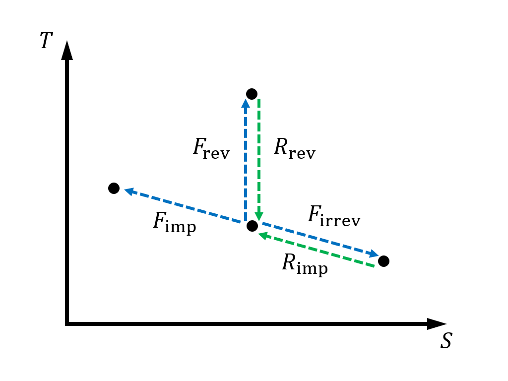
Since Q=0, there is no entropy convected into or out of the system. Therefore, the only contribution of entropy is \mathcal P_s. There are three situations to consider:
\Delta S<0: This requires \mathcal P_s<0, which is impossible since entropy cannot be destroyed.
\Delta S=0: This requires \mathcal P_s=0. These types of processes may occur in the forward or backwards direction (F and R both satisfy the requirement that entropy cannot be destroyed). As such, these processes are reversible.
\Delta S>0: This requires \mathcal P_s>0. These types of processes can only occur in the forward direction as R_{\mathrm{imp}} requires entropy destruction. As such, the reverse direction is impossible to occur and the process is irreversible.
All real processes are irreversible. Some processes may be minimally irreversible (i.e., close to the limit of reversibility). In these cases, the reversible assumption can be nearly correct and helpful as a limit.
Thermodynamic Definition of Temperature
Historically, temperature was assigned as a measurement of the degree of “hotness” of a substance. Maxwell, in the late 1800s, eventually introduced a thermodynamic definition for temperature based off mathematical reasoning.
We consider an isolated system C that is comprised of two closed systems A and B with differing temperatures. A rigid wall separates the two systems from one another. Since A and B are closed, they may exchange energy via heat transfer, but not mass. System C is retained by a rigid, adiabatic wall.
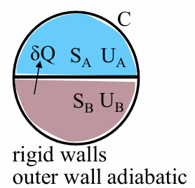
A and B are in internal thermodynamic equilibrium. They are not in thermodynamic equilibrium with each other as $T_A_B. Because of this, C is also not in thermodynamic equilibrium since its constituents are not in thermal equilibrium initially.
If we wait, we would expect the temperatures to equalize from heat transfer. When T_A=T_B, A and B are in thermal equilibrium with each other, so C is now in thermodynamic equilibrium. Since S_C can only increase, the maximum value of S_C occurs at thermal equilibrium when T_A=T_B and no more thermal change may occur.
For a nonreacting simple compressible substance
S_C=S_A(U_A, V_A)+S_B(U_B, V_B) \tag{1}
We arbitrarily choose U and V as two independent variables that S depends on. The choice of U and V is due to how the system is isolated and rigid, so \mathrm dU_C=0 and \mathrm dV=0.
Consider a progress variable \mu that tracks the fraction of U in A, \mu=U_A/U_C. Since V and U_C are fixed, the only variable that changes as the system equilibrates is \mu. If \mu=0, then all thermal energy in C is located in B. As \mu increases, S_C will increase until it equilibrates at some 0<\mu<1. Similarly, if \mu=1, all thermal energy in C is located in A and T_A will decrease until the equilibrium point. Therefore, the S-\mu graph will be an inverted parabolic shape. The equilibrium point occurs at the maximum.
We can find this equilibrium point by differentiating Eq. 1.
\frac {\mathrm dS_C}{\mathrm d\mu}=\left(\frac {\partial S_A}{\partial U_A}\right)_{V_A}\frac {\mathrm dU_A}{\mathrm d\mu}+\left(\frac {\partial S_B}{\partial U_B}\right)_{V_B}\frac {\mathrm dU_B}{\mathrm d\mu} \tag{2}
From the 1st and 2nd Laws for an isolated system at equilibrium, we also have
\begin{aligned} \frac {\mathrm dU_C}{\mathrm d\mu} & =\frac {\mathrm dU_A}{\mathrm d\mu}+\frac {\mathrm dU_B}{\mathrm d\mu}=0 \\ \frac {\mathrm dS_C}{\mathrm d\mu} & =0 \end{aligned}
Substituting into Eq. 2 gives
\left(\frac {\partial S_A}{\partial U_A}\right)_{V_A}=\left(\frac {\partial S_B}{\partial U_B}\right)_{V_B}
In other words, two systems are in thermal equilibrium when \left(\frac {\partial S}{\partial U}\right)_V is the same. However, by definition, we also know that two systems are in thermal equilibrium when T is the same. Therefore, we may use the derivative above to define T as
\boxed{T\equiv\left(\frac {\partial U}{\partial S}\right)_V} \tag{3}
The thermodynamic definition for temperature is only valid for nonreacting simple compressible substances in thermal equilibrium. This is because the only way for a temperature to be defined is if the system has a constant and uniformly distributed temperature. This is the only case for when T is “well-defined”.
The choice of T^{-1} for \left(\frac {\partial S}{\partial U}\right)_V is to ensure consistency with the definition that heat transfer occurs from high T to low T. If we assume T_A>T_B, then heat should flow from A to B. This means \mathrm dU_A<0. If we consider the total derivative of Eq. 1
\mathrm dS_C=\frac {\mathrm dU_A}{T_A}+\frac {\mathrm dU_B}{T_B}=\left(\frac 1{T_A}-\frac 1{T_B}\right)\,\mathrm dU_A
when T_A>T_B, \mathrm dU_A<0 as expected.
Thermodymamic Definition of Pressure
In a similar vein, pressure also has a thermodynamic definition. Instead of a rigid divider like in Sec. 3.2, we now use a flexible one that allows p_A and p_B to equalize. Though A and B are still closed, they may now exchange both Q and p\,\mathrm dV work.
This time, since the system may perform compression or expansion work, we must consider two progress variables \mu_U and \mu_V. Once again, at thermodynamic equilibrium, p_A=p_B and T_A=T_B
\frac {\mathrm dS_C}{\mathrm d\mu_U}=\frac {\mathrm dS_C}{\mathrm d\mu_V}=0
We differentiate Eq. 1 with respect to \mu_U and \mu_V to get
\begin{aligned} \frac {\mathrm dS_C}{\mathrm d\mu_U} & =\left(\frac {\partial S_A}{\partial U_A}\right)_{V_A}\frac {\mathrm dU_A}{\mathrm d\mu_U}+\left(\frac {\partial S_B}{\partial U_B}\right)_{V_B}\frac {\mathrm dU_B}{\mathrm d\mu_U}=\frac 1{T_A}\frac {\mathrm dU_A}{\mathrm d\mu_U}+\frac 1{T_B}\frac {\mathrm dU_B}{\mathrm d\mu_U} \\ \frac {\mathrm dS_C}{\mathrm d\mu_V} & =\left(\frac {\partial S_A}{\partial V_A}\right)_{U_A}\frac {\mathrm dV_A}{\mathrm d\mu_V}+\left(\frac {\partial S_B}{\partial V_B}\right)_{U_B}\frac {\mathrm dV_B}{\mathrm d\mu_V} \end{aligned}
The first equation is consistent with Eq. 2 for defining T. The second equation provides the condition for mechanical equilibrium as
\left(\frac {\partial S_A}{\partial V_A}\right)_{U_A}=\left(\frac {\partial S_B}{\partial V_B}\right)_{U_B}
To remain consistent with the fact that systems with higher p should expand against lower p, and the units of pressure as being Force/Length2, the thermodynamic definition for pressure is
\boxed{\frac pT\equiv\left(\frac {\partial S}{\partial V}\right)_U} \tag{4}
The thermodynamic definition for pressure is only valid for nonreacting simple compressible substances in thermodynamic equilibrium. The system must have a well-defined T, necessitating thermal equilibrium, and must also have a well-defined p, necessitating mechanical equilibrium.
Gibb’s Equation
Using Eq. 3 and Eq. 4 in our definition of S=S(U, V), then
\mathrm dS=\left(\frac {\partial S}{\partial U}\right)_V\,\mathrm dU+\left(\frac {\partial S}{\partial V}\right)_U\,\mathrm dV=\frac {\mathrm dU}T+\frac pT\,\mathrm dV
Re-arranging gives the classical form of Gibbs equation
\boxed{\mathrm dU=T\,\mathrm dS-p\,\mathrm dV} \tag{5}
This form of Gibb’s equation makes no assumption regarding the reversibility of any work processes, presence of heat transfer, etc. In fact, the only strict requirements are that the substance is a nonreacting simple incompressible substance and that the system is in thermodynamic equilibrium.
Heat Transfer and Entropy Transfer
Next, we investigate the relationship between heat transfer and entropy transfer. The relationship can be derived by considering a thermal energy reservoir (TER). This is a control mass whose thermal mass is large enough that heat transfer to or from the TER does not change its temperature. As such, we may assume our system’s T is constant and uniform (i.e., our system is always in thermodynamic equilibrium).
From Gibb’s equation with fixed volume and the 1st Law, we have
\mathrm dS=\frac {\mathrm dU}T=\frac {\delta Q}T \tag{6}
Heat Transfer and Entropy Production
At this point, we’ve established heat transfer can transfer entropy into or out of our system. However, entropy can also be produced. The conditions for entropy production only require a finite temperature difference to be present. To see why, we may consider an isolated system C that is comprised of two TERs, A and B. Without loss of generality, assume T_A>T_B and \delta Q flows from A into B.
From Sec. 3.5, \mathrm dS_A=-\frac {\delta Q}{T_A} and \mathrm dS_B=\frac {\delta Q}{T_B} so S_A must decrease as thermal energy flows from A to B. Conversely, S_B must increase since it receives energy from system A. To determine the entropy change for system B, we solve for \delta Q from system A’s entropy transfer and substitute into system B’s to get
\mathrm dS_B=-\frac {T_A}{T_B}\,\mathrm dS_A
Now, recall that system C is isolated. This means S_C must be constantly increasing until it reaches a maximum value at the thermal equilibrium point. Moreover, we can calculate the entropy contained in C by summing up the entropies contained in A and B! Doing so and taking the total derivative gives
\mathrm dS_C=\mathrm dS_A+\mathrm dS_B=\left(1-\frac {T_A}{T_B}\right)\,\mathrm dS_A\geq0
Entropy production occurs anytime there is heat transfer across a finite temperature difference. It is probably important to note that if a given amount of entropy leaves a system, this does not necessarily mean the same amount of entropy enters the surroundings. In simpler terms, if our system loses 400 J/K of entropy, this does not necessarily mean the surroundings then gain 400 J/K of entropy.
The reason for this is due to entropy production. If we consider the example above, then \mathrm dS_B=\frac {\delta Q}{T_B}>\frac {\delta Q}{T_A}=\mathrm dS_A. This means B receives more entropy than that leaving A since T_B<T_A. Since there was a finite temperature difference at the interface between A and B, entropy was produced!
Second Law for Control Mass
The total change in entropy for a control mass can be derived by considering an isolated system where a control mass receives energy from a TER and work is done to a mechanical energy reservoir (MER). Since the entire system is isolated, it may have entropy production \delta\mathcal P_s. The entropy production is equal to the entropy change gained from the TER and that lost to the MER.
\delta\mathcal P_s=\mathrm dS_{\mathrm{TER}}+\mathrm dS_{\mathrm{MER}}+\mathrm dS_{\mathrm{CM}}
For a control mass with no microscopic disorder (i.e., no entropy), the only possible way to exchange energy is through reversible work. Since there is no microscopic disorder, conductive heat transfer cannot occur as there is no gradient for energy to transfer along. Substituting in Eq. 6 gives
\mathrm dS_{\mathrm{CM}}=\frac {\delta Q}T+\mathcal P_s \tag{7}
The 1st and 2nd terms in the RHS of Eq. 7 are for entropy transferred and produced inside the control mass.
Recall that a reversible process is one where \mathcal P_s=0. For the case of Eq. 7, the system is reversible if \mathrm dS_{\mathrm{CM}}=\delta Q/T. If \mathrm dS_{\mathrm{CM}}>\delta Q/T, then the process must be irreversible.
Auxiliary Thermodynamic Functions
So far, we’ve been using the same set of thermodynamic properties for developing different relations. Certain quantities, like temperature, pressure, etc. can be easily measured. Other properties, however, like entropy and internal energy must be computed (entropy meters do not exist).
We may define any arbitrary thermodynamic property we choose, provided the units are consistent. In some cases, there are other properties that will be more convenient, depending on the situation, than the fundamental ones we’ve been using. Like internal energy, temperature, etc. these also have their own physical interpretations. Three very commonly used auxiliary properties are defined below; their extensive and intensive definitions are given respectively.
- Enthalpy
\begin{aligned} H & =U+pV \\ h & =u+pv \end{aligned} \tag{8}
- Gibbs Free Energy
\begin{aligned} G & =H-TS \\ g & =h-Ts \end{aligned} \tag{9}
- Helmholtz Free Energy
\begin{aligned} F & =U-TS \\ f & =u-Ts \end{aligned} \tag{10}
Properties of Enthalpy
To illustrate the advantage of enthalpy, consider a simple compressible substance that experiences a state change from state 1 to state 2. From its definition above, the enthalpy change \Delta H is
\Delta H_{12}=H_2-H_1=U_2-U_1+p_2V_2-p_1V_1=\Delta U_{12}+p_2V_2-p_1V_1
Now, let’s consider three different variations of a closed system (i.e., control mass). We consider the case of constant pressure (isobaric), constant volume (isochoric), and an isolated system (rigid and adiabatic). Recall that the substance is simple compressible, so the only significant reversible work mode is p\,\mathrm dV work. The 1st Law may be written as
\begin{aligned} \Delta U_{12} & =Q+W \\ \Delta H_{12} & =Q+W+p_2V_2-p_1V_1 \end{aligned}
Isobaric Process: Assuming p_1=p_2\equiv p, the 1st Law simplifies down to \Delta H_{12}=Q. In other words, the \Delta H of the system is equal to the heat transfer exchanged during the process.
Isochoric Process: If no volume change occurs, then \mathrm dV=0 and the 1st Law reduces down to \Delta U_{12}=Q. Here, internal energy change is a more useful property to use than enthalpy.
Isolated System: Since the system is isolated, energy and mass exchange are not permitted. From the 1st Law, that means \Delta U_{12}=0 so Q=W=0. Furthermore, because no work is permitted, the system’s volume must remain constant per \delta W=-p\,\mathrm dV. Therefore, the 1st Law becomes \Delta H_{12}=V\Delta p_{12}.
The three scenarios illustrate how H gives us an easy way to back out heat transfer for constant pressure systems by the 1st Law. If instead, the process is constant volume, then U should be used instead. And lastly, for the case of a rigid and adiabatic system, enthalpy is not “conserved” as its change depends on the pressure change across the processes.
Maxwell’s Relations and Mathematical Property Relationships
A useful skill to have is the ability to determine how various state properties change with respect to other quantities. So far, we’ve only investigated thermodynamic definitions for temperature, pressure, and chemical potential by writing them as partial derivatives between state properties. With the appropriate set of mathematical relations, we should be able to also express certain thermodynamic quantities in terms of partial derivatives and other thermodynamic quantities.
Let’s start off with Gibb’s equation. Recall Eq. 5 that expresses change in internal energy as a function of entropy and volumetric change. Written for a potentially reacting substance in intensive form, Eq. 5 becomes
\mathrm du=T\,\mathrm ds-p\,\mathrm dv+\sum\limits_i\mu_i\,\mathrm dn_i
We may use the various definitions for enthalpy, Gibbs free energy, and Helmholtz free energy to rewrite Eq. 5 in terms of those quantities.
\begin{aligned} h & =u+pv & \qquad\implies\qquad\mathrm dh & =T\,\mathrm ds+v\,\mathrm dp+\sum\limits_i\mu_i\,\mathrm dn_i \\ g & =h-Ts & \qquad\implies\qquad\mathrm dg & =-s\,\mathrm dT+v\,\mathrm dp+\sum\limits_i\mu_i\,\mathrm dn_i \\ f & =u-Ts & \qquad\implies\qquad\mathrm df & =-s\,\mathrm dT-p\,\mathrm dv+\sum\limits_i\mu_i\,\mathrm dn_i \end{aligned} \tag{11}
Recall that the mathematical definition of a total differential of f=f(x, y, z) is
\mathrm df=\frac {\partial f}{\partial x}\,\Biggr|_{y,z}\,\mathrm dx+\frac {\partial f}{\partial y}\,\Biggr|_{x,z}\,\mathrm dy+\frac {\partial f}{\partial z}\,\Biggr|_{x,y}\,\mathrm dz
Applying this on Eq. 11 allows us to express each differential coefficient in terms of partial derivatives. For each of these relations, we get the following:
\begin{aligned} T & =\left.\frac {\partial u}{\partial s}\,\right|_{v,n_i}=\left.\frac {\partial h}{\partial s}\,\right|_{p,n_i} & \qquad\qquad p & =\left.-\frac {\partial u}{\partial v}\,\right|_{s,n_i}=\left.-\frac {\partial f}{\partial v}\,\right|_{T,n_i} \\ v & =\left.\frac {\partial h}{\partial p}\,\right|_{s,n_i}=\left.\frac {\partial g}{\partial p}\,\right|_{T,n_i} & \qquad\qquad s & =\left.-\frac {\partial g}{\partial T}\,\right|_{p,n_i}=\left.-\frac {\partial f}{\partial T}\,\right|_{v,n_i} \end{aligned} \tag{12}
Van’t Hoff Relation
A useful application of Eq. 12 is the derivation of the van’t Hoff relation. Though not immediately applicable, we will use it later on for deriving an expression relating chemical equilibrium constants at different temperatures.
Consider the expression \left.\frac {\partial (G/T)}{\partial T}\right|_{p,n_i}. We may apply the quotient rule to express the derivative as
\begin{aligned} \left.\frac {\partial(G/T)}{\partial T}\right|_{p,n_i} & =\left.\frac {\partial G}{\partial T}\right|_{p,n_i}\frac 1T+G\left.\frac {\partial(1/T)}{\partial T}\right|_{p,n_i} \\ & =-\frac ST+G\left(-\frac 1{T^2}\right) \\ & =\frac {-G-TS}{T^2} \end{aligned}
Substitute the Gibbs free energy definition to see that
\boxed{\left.\frac {\partial(G/T)}{\partial T}\right|_{p,n_i}=-\frac H{T^2}} \tag{13}
This particular identity is useful since for an isothermal process, we can then relate the change between the two states using
\boxed{\left.\frac {\partial\left(\Delta G_{12}/T\right)}{\partial T}\right|_{p,n_i}=-\frac {\Delta H_{12}}{T^2}} \tag{14}
Maxwell’s Relations
With Eq. 12, we may construct more complex state property relations using a set of mathematical identities. For a sufficiently smooth and continuous function, whose derivatives up to the second derivative are well defined, the total derivative of F(y_1, y_2, \ldots, y_i) is
we have what’s known as the Reciprocity Rule. If we have the total derivative of , the total derivative gives
\begin{aligned} \mathrm dF & =\left.\frac {\partial F}{\partial y_1}\right|_{y_{j\neq1}}\,\mathrm dy_1+\left.\frac {\partial F}{\partial y_2}\right|_{y_{j\neq2}}\,\mathrm dy_2+\ldots+\left.\frac {\partial F}{\partial y_i}\right|_{y_{j\neq i}}\,\mathrm dy_i \\ & =x_1\,\mathrm dy_1+x_2\,\mathrm dy_2+\ldots+x_i\,\mathrm dy_i \end{aligned}
The Reciprocity Rule relates the derivatives of each coefficient x_j as
\boxed{\left.\frac {\partial x_i}{\partial y_j}\right|_{y_{k\neq j}}=\left.\frac {\partial x_j}{\partial y_i}\right|_{y_{k\neq i}}} \tag{15}
We may apply Eq. 15 to the left-hand side in each equation in Eq. 11 to show that
\begin{aligned} \left.\frac {\partial T}{\partial v}\right|_{s,n_i} & =-\left.\frac {\partial p}{\partial s}\right|_{v,n_i} & \qquad\qquad\left.\frac {\partial T}{\partial p}\right|_{s,n_i} & =\left.\frac {\partial v}{\partial s}\right|_{p,n_i} & \qquad\qquad\left.\frac {\partial\mu_i}{\partial p}\right|_{T,\chi_i,\chi_j} & =\left.\frac {\partial v}{\partial n_i}\right|_{T,p,n_{j\neq i}} \\ \left.\frac {\partial v}{\partial T}\right|_{p,n_i} & =\left.-\frac {\partial s}{\partial p}\right|_{T,n_i} & \qquad\qquad\left.\frac {\partial p}{\partial T}\right|_{v,n_i} & =\left.\frac {\partial s}{\partial v}\right|_{T,n_i} & \qquad\qquad\left.\frac {\partial\mu_i}{\partial T}\right|_{p,\chi_i,\chi_j} & =\left.-\frac {\partial s}{\partial n_i}\right|_{T,p,n_{j\neq i}} \end{aligned} \tag{16}
Since the relations in Eq. 16 were ultimately derived from various forms of Gibbs equations, the only assumption we’ve made is that the substance is a simple compressible substance.
A strong use case of Maxwell’s relations is creating equation-of-state relations by expressing a difficult-to-measure quantity like internal energy as a function of measureable properties. These measureable properties are typically p, T, and V. We illustrate with an example for internal energy, U.
For a nonreacting simple compressible substance, assume we can easily measure T and V. We may define U as a function of T and V and take the total derivative.
\mathrm dU=\left.\frac {\partial U}{\partial T}\right|_V\,\mathrm dT+\left.\frac {\partial U}{\partial V}\right|_T\,\mathrm dV
Substitute \mathrm dU into Eq. 5 and group common terms. By definition of the total derivative, then
\begin{aligned} \mathrm dS & =\frac 1T\,\mathrm dU+\frac pT\,\mathrm dV=\frac 1T\left(\left.\frac {\partial U}{\partial T}\right|_V\,\mathrm dT+\left.\frac {\partial U}{\partial V}\right|_T\,\mathrm dV\right)+\frac pT\,\mathrm dV \\ & =\underbrace{\frac 1T\left.\frac {\partial U}{\partial T}\right|_V}_{=\left.\partial S/\partial T\right|_V}\,\mathrm dT+\underbrace{\frac 1T\left(\left.\frac {\partial U}{\partial V}\right|_T+p\right)}_{=\left.\partial S/\partial V\right|_T}\,\mathrm dV \end{aligned}
Using Maxwell’s relations on the second coefficient, \left.\frac {\partial S}{\partial V}\right|_T=\left.\frac {\partial p}{\partial T}\right|_V, then we can express the derivative for U purely in terms of p and T.
\boxed{\left.\frac {\partial U}{\partial V}\right|_T=T\left.\frac {\partial p}{\partial T}\right|_V-p}
Variable Transformations
One last useful mathematical rule is called the cyclic rule, so called because the terms in a partial derivative, \left.\frac {\partial x}{\partial y}\right|_z can be “cyclically” rotated around to create a mathematical relation.
\boxed{\left.\frac {\partial x}{\partial y}\right|_z\left.\frac {\partial z}{\partial x}\right|_y\left.\frac {\partial y}{\partial z}\right|_x=-1} \tag{17}
Additionally, recall that the derivative is commutative for a continuous and existent derivative, and the inverse of a derivative is the same as inverting the “fraction” term inside the derivative.
\begin{aligned} \left.\frac {\partial x}{\partial y}\right|_z & =\left(\left.\frac {\partial y}{\partial x}\right|_z\right)^{-1} \\ \frac {\partial}{\partial z}\frac {\partial x}{\partial y} & =\frac {\partial^2x}{\partial z\partial y}=\frac {\partial}{\partial y}\frac {\partial x}{\partial z} \end{aligned}
Other Measurable Thermodynamic Quantities
We’ve currently established a list of thermodynamic properties that can be readily measured using a sensor or instrument. These properties are: p, T, V, and m. More broadly, however, there are other state properties that can be “easily” measured. The term “easily” in this case is relative, as each of the following properties require more work than the properties defined above, but measuring them in a lab setting is still certainly possible. They are
- Specific heats or heat capacities
- Heats of reaction or phase change
- Compressibility coefficients
We will see that each of these properties can be easily computed in a controlled setting based off their thermodynamic definitions. Each of these properties is measured in one of two ways.
- The amount of heat transfer, \delta Q, that takes place for one of the properties above to change
- The change in volume or density that occurs under a fixed condition (e.g., constant enthalpy).
Specific Heats
Writing out the internal energy and enthalpy of a closed system (control mass) as U=U(T, V) and H=H(T, p), the specific heats are defined as the change in either U or H based off the temperature change component.
\begin{aligned} \mathrm dU & =\left.\frac {\partial U}{\partial T}\right|_V\,\mathrm dT+\left.\frac {\partial U}{\partial V}\right|_T\,\mathrm dV\equiv C_V\,\mathrm dT+\left.\frac {\partial U}{\partial V}\right|_T\,\mathrm dV \\ \mathrm dH & =\left.\frac {\partial H}{\partial T}\right|_p\,\mathrm dT+\left.\frac {\partial H}{\partial p}\right|_T\,\mathrm dp\equiv C_p\,\mathrm dT+\left.\frac {\partial H}{\partial p}\right|_T\,\mathrm dp \end{aligned} \tag{18}
The subscripts denote the property held constant in the process. For C_V, this is defined as a change in U across a change in T at a fixed volume. Similarly, C_p is defined as a change in H across a change in T at fixed pressure. The properties defined above are extensive. We may relate them to their intensive counterparts by normalizing by mass or moles of substance.
Assume only p\,\mathrm dV work is allowed. The 1st Law applied to a control mass gives \mathrm dU=\delta Q-p\,\mathrm dV. If we further assume the process is isochoric or isobaric, then \mathrm dU and \mathrm dH in Eq. 18 becomes
\begin{aligned} \mathrm dU=\delta Q-p\,\mathrm dV & =C_V\,\mathrm dT & \qquad\implies\qquad C_V & =\frac {\delta Q}{\mathrm dT} \\ \mathrm dH=\mathrm dU+p\,\mathrm dV=\delta Q & =C_p\,\mathrm dT & \qquad\implies\qquad C_p & =\frac {\delta Q}{\mathrm dT} \end{aligned}
In other words, C_p and C_V simply indicate the amount of heat transfer required to change a substance’s temperature by \mathrm dT amount at constant pressure or constant volume respectively.
The definitions in Eq. 18 assume constant composition and constant phase where \mathrm dn_i=0. For this reason, Eq. 18 definitions should technically be called the frozen specific heats.
An important point regarding the definitions of C_p and C_V is that these quantities are not solely limited to cases where p or V are constant.
For example, let’s assume both T and p in a system changes across a process. There still exists a C_p quantity that can be used in the equation for \mathrm dH in Eq. 18. However, this quantity does not fully capture the enthalpy change as there is now a \left.\frac {\partial H}{\partial p}\right|_T component now.
\mathrm dH=C_p\,\mathrm dT+\left.\frac {\partial H}{\partial p}\right|_T\,\mathrm dp\neq C_p\,\mathrm dT
Since state properties are path independent, we may consider the process as having two contributions. The first contribution is an isobaric process, as indicated by the \mathrm dT term, and the second contribution is an isothermal process, as indicated by the \mathrm dp term. Upon adding the two contributions, we arrive at the same final state as the original process.
From Eq. 16, we can show that
\begin{aligned} &\boxed{ \phantom{C_V}\mathllap{C_V} = \mathrlap{ \left.\frac{\partial U}{\partial T}\right|_V = T\left.\frac{\partial S}{\partial T}\right|_V } \phantom{ \left.\frac{\partial H}{\partial T}\right|_V = T\left.\frac{\partial S}{\partial T}\right|_V } } \\[0.5em] &\boxed{ \phantom{C_V}\mathllap{C_p} = \mathrlap{ \left.\frac{\partial H}{\partial T}\right|_p = T\left.\frac{\partial S}{\partial T}\right|_p } \phantom{ \left.\frac{\partial H}{\partial T}\right|_V = T\left.\frac{\partial S}{\partial T}\right|_V } } \end{aligned} \tag{19}
Though the partial derivative definitions for C_V and C_p are rooted in pure mathematics, the results from the application of Maxwell’s relations assume the substance is a nonreacting simple compressible substance.
Compressibility Coefficients
Assume the substance in thermodynamic equilibrium obeys a p-v-T equation of state. Moreover, we assume that volume is expressed in terms of T and p as V=V(T, p). The total derivative definition gives
\mathrm dV=\left.\frac {\partial V}{\partial T}\right|_p\,\mathrm dT+\left.\frac {\partial V}{\partial p}\right|_T\,\mathrm dp\equiv\alpha V\,\mathrm dT-\kappa V\,\mathrm dp
This leads to the definitions of the isobaric compressibility coefficient \alpha and the isothermal compressibility coefficient \kappa. We also have, distantly, the isentropic compressibility coefficient \beta.
\begin{aligned} &\boxed{ \phantom{\alpha}\mathllap{\alpha} \equiv \mathrlap{ \frac{1}{V} \left.\frac{\partial V}{\partial T}\right|_p } \phantom{ -\frac{1}{V} \left.\frac{\partial V}{\partial p}\right|_T } } \\[0.5em] &\boxed{ \phantom{\alpha}\mathllap{\kappa} \equiv \mathrlap{ -\frac{1}{V} \left.\frac{\partial V}{\partial p}\right|_T } \phantom{ -\frac{1}{V} \left.\frac{\partial V}{\partial p}\right|_T } } \\[0.5em] &\boxed{ \phantom{\alpha}\mathllap{\beta} \equiv \mathrlap{ -\frac{1}{V} \left.\frac{\partial V}{\partial p}\right|_S } \phantom{ -\frac{1}{V} \left.\frac{\partial V}{\partial p}\right|_T } } \end{aligned} \tag{20}
Most texts and literature papers reverse the definitions of \alpha and \beta above in Eq. 20. That is, \alpha is defined as the isentropic compressibility coefficient and \beta is the isobaric compressibility coefficient. Be sure to consult the notation used in each text for consistency. This course and document assumes the definitions given in Eq. 20.
The equations in Eq. 20 require a state equation to be supplied. We can illustrate calculating \alpha and \kappa through the p-v-T equation with the ideal gas law.
For a nonreacting, thermally perfect, ideal gas in thermodynamic equilibrium, \alpha and \kappa take on simple expressions.
\begin{aligned} \alpha & =\frac 1V\textcolor{red}{\left.\frac {\partial V}{\partial T}\right|_p}=\frac 1V\frac {n\overline R}p\boxed{=\frac 1T}\\ \beta & =-\frac 1V\textcolor{red}{\left.\frac {\partial V}{\partial p}\right|_T}=\frac 1V\frac {n\overline RT}{p^2}\boxed{=\frac 1p} \end{aligned}
We can also apply Eq. 15 to the governing \mathrm dV equation to derive a differential relation between \alpha and \kappa.
\boxed{\left.\frac {\partial\alpha}{\partial p}\right|_T=\left.-\frac {\partial\kappa}{\partial T}\right|_p} \tag{21}
And from the cyclic rule, Eq. 17, with (x, y, z)=(p, T, V), then \alpha and \kappa are related by the following derivative:
\boxed{\left.\frac {\partial p}{\partial T}\right|_V=\frac {\alpha}{\kappa}} \tag{22}
Specific Heats and Compressibility Coefficient Relationship
For a nonreacting simple compressible substance, C_p and C_V are related by the compressibility coefficients.
\boxed{C_p-C_V=TV\frac {\alpha^2}{\kappa}} \tag{23}
If we further make the assumption that the substance is a thermally perfect gas, then \alpha=\frac 1T and \kappa=\frac 1p so Eq. 23 reduces down to
\hat c_p-\hat c_V=\overline R
Note that the C_p and C_V quantities are the per-molar intensive quantities of the substance and \overline R is the universal gas constant.
General Conditions for Chemical Equilibrium
The remaining two auxiliary properties, G and F, are more useful for describing the point where a mixture reaches chemical equilibrium. To set the context, imagine we have a mixture enclosed by our system boundary. Depending on the composition of each species, this mixture may or may not be in chemical equilibrium. In some cases, we may be interested at the chemical equilibrium point, where the relative compositions of each species stabilizes within a certain time frame.
To illustrate the usefulness of G and F, we consider the case where there is no work except p\,\mathrm dV work. Writing the 1st and 2nd Laws out, we have
\begin{aligned} \mathrm dU & =\delta Q+\delta W=\delta Q-p\,\mathrm dV \\ \mathrm dS & =\frac {\delta Q}T+\delta\mathcal P_s \end{aligned}
Solving for \delta Q in the 1st Law and substituting into the 2nd Law gives an equation similar in form to Eq. 5. We’ve made no assumptions regarding the reversibility of the process.
T\,\mathrm dS-\mathrm dU-p\,\mathrm dV=\delta\mathcal P_s\geq0
Once again, we consider the three scenarios for an isolated system, a system undergoing a constant T and V process, and a system undergoing a constant T and p process.
Isolated System: Since \mathrm dU=\mathrm dV=0 (see Sec. 4.1 for why), the equation above reduces down to \mathrm dS\geq0. In other words, as the mixture tends towards chemical equilibrium, the entropy continues increasing until it is maximized at the equilibrium point.
Constant T and V System: Since \mathrm dT=\mathrm dV=0, we can show that
T\,\mathrm dS-\mathrm dU-p\,\mathrm dV=\mathrm d(U-TS)-S\,\mathrm dT-p\,\mathrm dV=-\mathrm dF\geq 0
Therefore, \mathrm dF\leq0 and the Helmholtz free energy is minimized at the equilibrium point. This minimization, however, is only appropriate for systems at constant temperature and volume.
Constant T and p System: Since \mathrm dT=\mathrm dp=0, we can show similarly that
T\,\mathrm dS-\mathrm dU-p\,\mathrm dV=T\,\mathrm dS-\mathrm d(U+pV)+V\,\mathrm dp=\mathrm d(TS-H)-S\,\mathrm dT+V\, \mathrm dp=-\mathrm dG\geq0
Therefore, \mathrm dG\leq0 and Gibbs free energy is also minimized at the equilibrium point.
To determine when a mixture is in chemical equilibrium, we may look at the free energy available depending on the system and what thermodynamic properties are being kept constant. For an isolated system with constant U and V, the chemical equilibrium point occurs where entropy is maximized. This matches the process used when deriving Eq. 3 and Eq. 4 in Sec. 3.2 and Sec. 3.3.
\mathrm dS\geq0
Meanwhile, for an isothermal and isochoric system (constant T and V), chemical equilibrium can be determined by finding the composition that minimizes the Helmholtz free energy.
\mathrm dF\leq0
And lastly, for an isothermal and isobaric system (constant T and p), the composition that minimizes the Gibbs free energy determines the chemical equilibrium point.
\mathrm dG\leq0
The scenarios above each made assumptions regarding the process that occurred to reach the chemical equilibrium point. For Helmholtz energy, for instance, we restricted T and V to be constant in the process. This is akin to leaving this mixture in a rigid and isothermal box, while letting its composition vary until the equilibrium point is reached.
These restrictions, if they must be strictly enforced, render the relations above useless. For most engineering applications, especially in aerospace, constant T and V or constant T and p never occur. In fact, constant temperature and pressure in a rocket engine typically indicates poor operating efficiency! Fortunately for us, the actual process doesn’t have to take place at these restricted conditions to be able to use these relations. For instance, we may still apply the concept of minimizing Gibbs free energy, G, in a mixture, if the mixture’s T and p are known! This is what makes Gibbs free energy particularly useful, as it is very easy for us to measure a fluid’s temperature and pressure. Once the fluid state is known, the problem is simply an optimization problem to determine the point of G_{\mathrm{min}}!
Chemical Potential and Mixture Equilibria
The substances we’ve considered up until this point have been pure substances (single species). We’ve defined our thermodynamic properties as a function of two other independent thermodynamic properties, e.g., S=S(U, V). Now, we expand our consideration to include mixtures of k simple compressible substances. For mixtures, the composition must also be known to determine whether two thermodynamic states are identical. With entropy, for example, we must now have
S=S(U, V, n_1, n_2, \ldots, n_k)
Using the thermodynamic definitions of temperature and pressure (Eq. 3 and Eq. 4) on the total derivative of S, and assuming the system is in thermal and mechanical equilibrium, gives
\mathrm dS=\left(\frac {\partial S}{\partial U}\right)_{V,n_i}\,\mathrm dU+\left(\frac {\partial S}{\partial V}\right)_{U,n_i}\,\mathrm dV+\sum\limits_{j=1}^k\left(\frac {\partial S}{\partial n_j}\right)_{U,V,n_{i\neq j}}\,\mathrm dn_j=\frac {\mathrm dU}T+\frac pT\,\mathrm dV-\frac 1T\sum\limits_{j=1}^k\mu_j\,\mathrm dn_j
The index variable 1\leq i\leq k accounts for all constituents inside the mixture. The notation n_i means the set of moles of species i where 1\leq i\leq k. On its own, n_i refers to the moles of each species, for all species in the mixture. And when n_{i\neq j} like in the sum, we effectively exclude the number of moles of species j from the set.
The last partial derivative T\left(\partial S/\partial n_j\right)_{U,V,n_{i\neq j}} is defined as the chemical potential \mu_j. The mathematical definition effectively accounts for the entropy change when the number of moles of species j is varied with everything else constant. Note that this property is a molar intensive property since it’s the extensive entropy change, \partial S, normalized by the number of moles n_j. Its units, therefore, are Energy/Moles.
With thermal and mechanical equilibriums, we said that two systems have the same T and p respectively assuming no external and body forces act on the system. Therefore, it stands to reason that two systems in chemical and phase equilibrium must have the same \mu. For example, when freezing water at 0^{\circ}C, the chemical potentials between the two phases (ice and water) will be identical: \mu_{\mathrm{liq}}=\mu_{\mathrm{ice}}. Similarly, for a chemical reaction like
\mathrm N_2+\mathrm O_2\rightleftharpoons2\mathrm{NO}
the total chemical potential of the reactants’ side should be equal to that of the product’s side at chemical equilibrium. The total chemical potential of a species is given by the product of the species’ \mu and the number of moles of that species. Therefore, \mu_{\mathrm N_2}+\mu_{\mathrm O_2}=2\mu_{\mathrm{NO}} in the equation above.
Equilibrium States for Reacting Gases
Now we shift our focus to chemical equilibrium. The goal for this section is how to determine the chemical equilibrium state of a mixture of gases when the thermodynamic state and initial mixture are known.
Recall from the state postulate that it takes two independent, intensive thermodynamic properties to be known for a well-defined simple compressible substance to uniquely constrain its state. In general, for gases, the common pairs of thermodynamic properties we choose are (u, v), (h, p), or (T, p). For our example, as well as most applications we will see, it is generally common to specify (T, p) for the mixture.
However, knowing the two thermodynamic properties alone is not enough. Remember, the state postulate requires the substance to be well-defined. We generally do not know the composition of the mixture at chemical equilibrium and therefore, the crux of the problem now boils down to ways of determining the equilibrium composition when two independent properties are known.
Fortunately though, the equilibrium composition is uniquely determined by the relative amount of initial masses present due to mass conservation. Because we cannot create nor destroy nuclei, mass conservation requires the number of atomic nuclei in the equilibrated state be equal to the amount of atomic nuclei in the initial state. For example, if we consider a mixture initially consisting of 5 moles of \mathrm{NH_3} and 8 moles of \mathrm{N_2O}, we know the equilibrium composition must contain \mathrm N:\mathrm H:\mathrm O in a 21:15:8 ratio as it is physically impossible to have an \mathrm H atom convert into an \mathrm N atom in the absence of nuclear reactions.
When calculating the equilibrium state of a mixture of reacting gases, it is enough to specify the atomic ratios of the initial mixture to constrain the equilibriated substance. That is, simply knowing the number of atoms total in the mixture is enough to classify the substance as “well-defined”. It is not necessary to know the exact species and their amounts in the initial mixture.
With the thermodynamic state known, we may proceed with determining the equilibrium composition. Recall that a general requirement for equilibrium is that
\sum\limits_i\mu_i\,\mathrm dn_i=0 \tag{24}
This is true regardless if we assume the mixture is thermally perfect, ideal, calorically perfect, etc. Additionally, recall in Sec. 4, we concluded that if T and p are known, we may determine the equilibrium point as the point where G of the mixture is minimized.
Chemical Reaction Review
Before proceeding, it is helpful to review some useful concepts related to chemical equilibrium. Recall that for a balanced chemical reaction, we require
\sum\limits_i \nu_iM_i=0 \tag{25}
where \nu_i is the stoichiometric coefficient of the ith species, M_i. By definition, \nu_i>0 for species on the right-hand side, and negative for species on the left-hand side.
The notation used in Eq. 25 may seem confusing initially, but interpreting the summation term-by-term shows that Eq. 25 is an alternate way of writing any chemical relation. For each species in the chemical relation, we multiply by its signed coefficient and add everything together. If the equation is properly balanced, the right-hand side should be zero. This is equivalent to writing the chemical relation as a mathematical equation where all species on the left-hand side have been moved to the right-hand side.
For example, the balanced chemical reaction for the formation of water vapor is
\mathrm{H_2}+\frac 12\mathrm{O_2}\rightleftharpoons\mathrm{H_2O}
Therefore, 1\leq i\leq 3 and we have the following relation from Eq. 25.
\sum\limits_i\nu_iM_i=1\cdot\mathrm{H_2O}+(-1)\cdot\mathrm{H_2}+\left(-\frac 12\right)\cdot\mathrm{O_2}=\mathrm{H_2O}-\mathrm{H_2}-\frac 12\mathrm{O_2}=0
The last equation is equivalent to the \mathrm{H_2O} formation equation we wrote above, but with all species moved to the same side and the \rightleftharpoons replaced with an equals sign!
We may define the progress variable \mathrm dn for species i as so.
\mathrm dn=\frac {\mathrm dn_i}{\nu_i} \tag{26}
When the reaction proceeds towards the right-hand side, \mathrm dn>0. Conversely, when the reaction proceeds towards the left-hand side, \mathrm dn<0.
To see why \mathrm dn>0 or \mathrm dn<0 automatically determines the “favored” direction, we apply Eq. 26 to a product and reactant for a reaction proceeding to the right and show the sign is the same.
To do so, we first assume species i is a product. When the reaction shifts to the right, \mathrm dn_i>0 as more molecules of species i are formed. Since \nu_i>0 as the molecule is on the right-hand side, the division in Eq. 26 is positive and \mathrm dn>0.
Now, we assume species i is a reactant. When the reaction shifts to the right, \mathrm dn_i<0 as molecules of species i are consumed to form more products. This time, \nu_i<0 as i is on the left-hand side, so Eq. 26 remains \mathrm dn>0.
The case where the reaction proceeds to the left is identical to the right-direction shift considered above, except the signs are inverted and \mathrm dn<0 regardless if species i is a product or reactant.
Substitute Eq. 26 into the differential form of Eq. 24 like so.
\mathrm dG=\sum\limits_i\mu_i\,\mathrm dn_i=\sum\limits_i\nu_i\mu_i\,\mathrm dn\leq0 \tag{27}
Since G reaches a minimum at chemical equilibrium, the derivative must be zero at that point.
Let’s consider the case for a thermally perfect gas. From eq. XXX, G becomes
\begin{aligned} G=\sum\limits_i\mu_in_i & =\sum\limits_in_i\left[\mu_i^0+\overline RT\ln\left(\frac p{p^0}\right)\right] \\ & =\sum\limits_in_i\left[\mu_i^0+\overline RT\ln\left(\frac p{p^0}\right)+\overline RT\ln\chi_i\right] \\ & =\sum\limits_in_i\mu_i^0+\sum\limits_in_i\overline RT\ln\chi_i \end{aligned}
We assume fixed temperature, T, in the last equation and evaluated the system pressure at standard pressure, p=p^0. The first term involving \mu_i^0 is only a function of T as \mu_i^0 is always evaluated at standard pressure. Thus, the first term accounts for the change in G due to changes in T.
The second term accounts for the
When both terms strike a balance and minimize G, that is when the equilibrium point occurs.
Equilibrium Constant for Thermally Perfect Gas
We look at the case for a thermally perfect gas. From eq. XXX, we know that the chemical potential for a thermally perfect gas can be separated into a temperature and pressure dependence.
\mu_i=\mu_i^0+\overline RT\ln\left(\frac p{p^0}\right)
At equilibrium, we know that \sum\limits_i\nu_i\mu_i^*=0. The * denotes conditions at chemical equilibrium. Substituting the equation above into the condition for equilibrium, we may define a new thermodynamic property called the equilibrium constant, K_p.
\boxed{-\frac 1{\overline RT}\sum\limits_i\nu_i\mu_i^0=\ln\prod\limits_i\left(p_i^*\right)^{\nu_i}\equiv\ln K_p}
Rewrite to solve for K_p gives
K_p\equiv\prod\limits_i\left(p_i^*\right)^{\nu_i}=\exp\left(-\frac 1{\overline RT}\sum\limits_i\nu_i\mu_i^0\right) \tag{28}
Start with the Gibbs free energy at the equilibrium point and substitute the chemical potential in.
\sum\limits_i\nu_i\mu_i^*=\sum\limits_i\nu_i\left[\mu_i^0+\overline RT\ln\left(\frac {p_i^*}{p^0}\right)\right]=0
Distribute the sum and separate the pressure-dependent term from the temperature-dependent term.
-\frac 1{\overline RT}\sum\limits_i\nu_i\mu_i^0=\sum\limits_i\nu_i\ln\left(\frac {p_i^*}{p^0}\right)=\sum\limits_i\ln\left[\left(\frac {p_i^*}{p^0}\right)^{\nu_i}\right]
Recall that a sum of logarithms can be collapsed into a single logarithm.
\ln x_1+\ln x_2+\ldots+\ln x_n=\sum\limits_{i=1}^n\ln x_i=\ln(x_1x_2\ldots x_n)=\ln\prod\limits_{i=1}^nx_i
Applying this identity and defining K_p as the quantity inside the natural logarithm, Eq. 28 naturally falls out.