Part C: Reflection and Transmission of Waves
Fluid-Fluid Boundaries
Normal Incidence
Consider the case where an incident plane wave with pressure p_i colliding with a fluid-fluid boundary. The fluids have different characteristic impedances. That is, z_{0,1}\neq z_{0,2}.
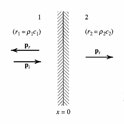
Part of the wave is transmitted through the boundary into medium 2. We denote this wave with p_t to signify that it is transmitted through the boundary. Another part of the incident wave is reflected by the boundary back into medium 1. Let p_r denote the reflected wave. The goal is to determine how much of p_i is transmitted vs. reflected.
Define the pressure reflection coefficient as the ratio between the reflected wave’s pressure to that of the incident wave’s. We may define an identical quantity for the transmitted pressure, called the pressure transmission coefficient.
\begin{aligned} \underline T & =\frac {\underline{\underline p}_t}{\underline{\underline p}_i} \\ \underline R & =\frac {\underline{\underline p}_r}{\underline{\underline p}_i} \end{aligned} \tag{1}
These two quantities are currently unknown, so we need a total of 2 equations. These two equations come from conservation laws. We have that at the boundary, the net force from the incident wave “colliding” with the boundary should be zero to prevent the boundary from moving (the boundary does not accelerate nor move with constant velocity). Therefore, pressure must be continuous across the boundary.
p_1(0, t)=p_2(0, t) \tag{2}
The second constraint is that the particle velocities must be equal on both sides as energy is transferred across the boundary, but mass is not.
\underline{\mathbf u}_1=\underline{\mathbf u}_2 \tag{3}
Pressure Continuity Constraint
We may express \underline p_i, \underline p_t, and \underline p_r using their harmonic plane wave definitions.
\begin{aligned} \underline p_i(x, t) & =\underline{\underline p}_i e^{j(\omega t-k_1x)} \\ \underline p_t(x, t) & =\underline{\underline p}_t e^{j(\omega t-k_2x)} \\ \underline p_r(x, t) & =\underline{\underline p}_r e^{j(\omega t+k_1x)} \end{aligned} \tag{4}
The pressure in medium 1 is the sum of \underline p_i and \underline p_r. And the pressure in medium 2 is simply \underline p_t. Therefore, Eq. 2 becomes
\underline{\underline p}_i+\underline{\underline p}_r=\underline{\underline p}_t
Normalize both sides by \underline{\underline p}_t to recover \underline T and \underline R.
\boxed{1+\underline R=\underline T} \tag{5}
Particle Velocity Constraint
From the equation of \underline{\mathbf u} for a plane wave, we have the following
\begin{aligned} \underline u_i(x, t) & =\frac {\underline{\underline p}_i(x, t)}{\rho_1c_1}e^{j(\omega t-k_1x)} \\ \underline u_t(x, t) & =\frac {\underline{\underline p}_t(x, t)}{\rho_2c_2}e^{j(\omega t-k_2x)} \\ \underline u_r(x, t) & =-\frac {\underline{\underline p}_r(x, t)}{\rho_1c_1}e^{j(\omega t+k_1x)} \end{aligned} \tag{6}
The particle velocity in fluid 1 is the sum of the incident and reflected particle velocities. And the particle velocity in fluid 2 is simply that of the transmitted wave’s. Therefore, Eq. 3 becomes
\frac {\underline{\underline p}_i-\underline{\underline p}_r}{\rho_1c_1}=\frac {\underline{\underline p}_t}{\rho_2c_2}
Dividing both sides by \underline{\underline p}_i, we get
\frac {1-\underline R}{z_1}=\frac {\underline T}{z_2} \tag{7}
Transmission and Reflection Coefficients
With Eq. 5 and Eq. 7, solving for \underline T and \underline R gives
\begin{aligned} &\boxed{ \mathrlap{\underline{T}=\frac{2z_2}{z_1+z_2}=\frac{2z_2/z_1}{1+z_2/z_1}} \phantom{\underline{R}=\frac{z_2-z_1}{z_1+z_2}=\frac{z_2/z_1-1}{1+z_2/z_1}} }\\[8pt] &\boxed{ \underline{R}=\frac{z_2-z_1}{z_1+z_2}=\frac{z_2/z_1-1}{1+z_2/z_1} } \end{aligned} \tag{8}
Let’s now investigate specific cases of reflection and transmissions across the boundary.
Case 1: z_1\ll z_2
An example of z_1\ll z_2 is an incident wave propagating from air into water. In Eq. 8, we assume z_2 contribution is negligible so \underline T=2 and \underline R=1. Under these conditions, the transmitted pressure is expected to be twice as large as that of the incident wave. And the reflected pressure amplitude is expected to be equal to that of the incident wave.
Case 2: z_1\gg z_2
For the opposite case, where a wave is propagating from water into air, we assume that the impedance z_2 is negligible in Eq. 8 so \underline T=\frac {2z_2}{z_1}\ll 1 and \underline R=-1. The transmitted wave amplitude is very small (seemingly negligible), whereas the reflected wave amplitude is equal in magnitude to the incident wave’s, but opposite in phase.
Intensity Transmission and Reflection Coefficients
The time-averaged intensities can be constructed in an identical manner to \underline T and \underline R.
\begin{aligned} T_I & =\frac {I_t}{I_i} \\ R_I & =\frac {I_r}{I_i} \end{aligned}
From the acoustic intensity formulas for a plane wave, we have
\begin{aligned} I_i & =\frac {\left|\underline p_i\right|^2}{2z_1} \\ I_t & =\frac {\left|\underline p_t\right|^2}{2z_2} \\ I_r & =\frac {\left|\underline p_r\right|^2}{2z_1} \end{aligned} \tag{9}
For the reflection coefficient, the two impedances cancel as they’re both z_1. The transmission coefficient, on the other hand, includes a \frac {z_2}{z_1} ratio. Simplification gives
\begin{aligned} &\boxed{ \mathrlap{R_I=\left|\underline R\right|^2=\left(\frac{z_2-z_1}{z_2+z_1}\right)^2} \phantom{T_I=\frac{z_2}{z_1}\left|\underline T\right|^2=\frac{4z_1z_2}{(z_1+z_2)^2}} }\\[8pt] &\boxed{ T_I=\frac{z_2}{z_1}\left|\underline T\right|^2=\frac{4z_1z_2}{(z_1+z_2)^2} } \end{aligned} \tag{10}
Case 1: z_1\ll z_2
We consider z_1 negligible compared to z_2. The intensity transmission coefficient becomes
T_I=\frac {4z_1z_2}{(z_1+z_2)^2}\approx\frac {4z_1}{z_2}\ll1
In Sec. 1.1.3.1, we computed \underline T\simeq2 and \underline R\simeq1, meaning the transmitted wave’s pressure amplitude was doubled while the reflected wave’s amplitude remained constant. Despite having a \underline T=2, T_I\ll1 meaning the acoustic power is very small.
This is a consequence of the high impedance in medium 2. The impedance scales as \underline z=\frac {\underline p(x, t)}{\underline{\mathbf u}(x, t)}. Even though the pressure amplitude is doubled, because of the high impedance, the particle velocity is still very small in medium 2. As a result, the power transmitted is still very small despite the high pressure.
This type of boundary, where the impedance increases from low to high across the interface, is often referred to as a hard boundary or a rigid wall.
Case 2: z_1\gg z_2
We consider z_2 to be negligible compared to z_1. The intensity transmission coefficient becomes
T_I=\frac {4z_1z_2}{(z_1+z_2)^2}\approx\frac {4z_2}{z_1}\gg1
In Sec. 1.1.3.2, we determined \underline T\simeq0 and \underline R\simeq-1. Since \underline T\simeq0, there is no transmitted wave through medium 2. Moreover, the reflected wave in medium 1 has the same pressure amplitude as the incident wave, but is out of phase by \pi. The two waves destructively intefere and cancel each other out exactly. The total response in fluid 1 is a standing wave.
This type of boundary, where the impedance increases from high to low across the boundary, is called a pressure release boundary since the acoustic pressure disappears through the interface.
Power Transmission and Reflection Coefficients
Since there is a relation between \mathbf I and \Pi, we may also construct power transmission and reflection coefficients for each wave. If we define S to be the cross-sectional area of the wave, then \Pi=SI. From conservation of power, we have
\Pi_i=\Pi_r+\Pi_t
That is, the incident wave carries all the power prior to the exchange. Normalize both sides by \Pi_i to obtain
R_{\Pi}+T_{\Pi}=1 \tag{11}
Since S is constant for the incident, transmitted, and reflected waves, we also have the same relation for acoustic intensity. That is
I_i=I_r+I_t \tag{12}
Therefore, for normal incidence, the power and intensity coefficients have the same formulas.
\begin{aligned} &\boxed{ \mathrlap{T_{\Pi}=T_I=\frac{4z_1z_2}{(z_1+z_2)^2}} \phantom{R_{\Pi}=R_I=\left(\frac{z_2-z_1}{z_2+z_1}\right)^2} }\\[8pt] &\boxed{ R_{\Pi}=R_I=\left(\frac{z_2-z_1}{z_2+z_1}\right)^2 } \end{aligned} \tag{13}
From Eq. 12 or Eq. 11, since the incident beam carries the entire intensity and power, we have that
\begin{gathered} 0\leq T_I\leq1 \\ 0\leq R_I\leq1 \end{gathered}
The same set of restrictions apply for T_{\Pi} and R_{\Pi}.
Normal Incidence on Fluid Layer
Now, we extend the derivation to include a layer of fluid, referred to as medium 2, that separates media 1 and 3 from each other. An incident plane wave propagates through medium 1 and must travel through two boundaries to reach fluid 3, as shown in Fig. 1.
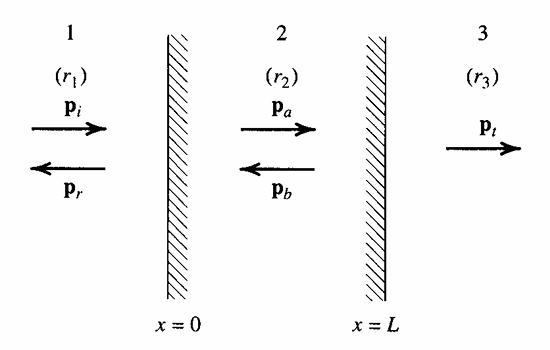
As \underline p_i reaches the boundary between fluid 1 and 2, it will separate into a transmitted and reflected wave labeled \underline p_a and \underline p_r respectively in Fig. 1. Similarly, as \underline p_a reaches the boundary between fluid 2 and 3, it too will be decomposed into a transmitted and reflected component labeled \underline p_t and \underline p_b. We assume the fluid layer has length L with the left-side interface positioned at x=0.
Constraints
Like the normal incidence on a fluid boundary, we must ensure continuous pressure and particle velocity across the boundary. That is, the pressure and particle velocities on either side must be equal. These serve as the boundary conditions that allow us to compute \underline T, \underline R, T_I, R_I, and so on.
Continuity of Pressure
The harmonic pressure equations for the pressures in all three fluids are
\begin{aligned} \underline p_1(x, t) & =\underline p_i(x, t)+\underline p_r(x, t)=\underline{\underline p}_ie^{j(\omega t-k_1x)}+\underline{\underline p}_re^{j(\omega t+k_2x)} \\ \underline p_2(x, t) & =\underline p_a(x, t)+\underline p_b(x, t)=\underline Ae^{j(\omega t-k_2x)}+\underline Be^{j(\omega t+k_2x)} \\ \underline p_3(x, t) & =\underline p_t(x, t)=\underline{\underline p}_te^{j(\omega t-k_3x)} \end{aligned} \tag{14}
Since there are two boundaries, we now have two sets of equations for continuity of pressure alone.
\begin{gathered} \underline{\underline p}_i+\underline{\underline p}_r=\underline A+\underline B \\ \underline Ae^{-jk_2L}+\underline Be^{jk_2L}=\underline{\underline p}_te^{-jk_3L} \end{gathered} \tag{15}
Continuity of Particle Velocities
Similar to Eq. 15, we may also write two sets of equations for the particle velocities. From the particle velocity equation for a plane wave, we have
\begin{aligned} \underline u_1(x, t) & =\underline u_i(x, t)+\underline u_r(x, t)=\frac {\underline{\underline p}_i }{z_1}e^{j(\omega t-k_1x)}-\frac {\underline{\underline p}_r}{z_1}e^{j(\omega t+k_1x)} \\ \underline u_2(x, t) & =\underline u_A(x, t)+\underline u_B(x, t)=\frac {\underline A}{z_1}e^{j(\omega t-k_2x)}-\frac {\underline B}{z_2}e^{j(\omega t+k_2x)} \\ \underline u_3(x, t) & =\frac {\underline p_t(x, t)}{z_3}=\frac {\underline{\underline p}_t}{z_3}e^{j(\omega t-k_3x)} \end{aligned} \tag{16}
Continuity of particle velocity applied to x=0 and x=L interfaces gives
\begin{gathered} \frac {\underline{\underline p}_i-\underline{\underline p}_r}{z_1}=\frac {\underline A-\underline B}{z_2} \\ \frac {\underline A}{z_2}e^{-jk_2L}-\frac {\underline B}{z_2}e^{jk_2L}=\frac {\underline{\underline p}_t}{z_3}e^{-jk_3L} \end{gathered} \tag{17}
Transmission and Reflection Coefficients
Together, Eq. 15 and Eq. 17 give four equations for four unknowns: \underline T, \underline R, \underline A/\underline{\underline p}_i, and \underline B/\underline{\underline p}_i. Solving for \underline T and \underline R gives
\begin{aligned} &\boxed{ \mathrlap{\underline T=\frac{2}{(1+z_1/z_3)\cos k_2L+j(z_2/z_3+z_1/z_2)\sin k_2L}} \phantom{\underline R=\frac{(1-z_1/z_3)\cos k_2L+j(z_2/z_3-z_1/z_2)\sin k_2L}{(1+z_1/z_3)\cos k_2L+j(z_2/z_3+z_1/z_2)\sin k_2L}} }\\[8pt] &\boxed{ \underline R=\frac{(1-z_1/z_3)\cos k_2L+j(z_2/z_3-z_1/z_2)\sin k_2L}{(1+z_1/z_3)\cos k_2L+j(z_2/z_3+z_1/z_2)\sin k_2L} } \end{aligned} \tag{18}
The transmitted and reflection coefficients can be related to one another, similar to Eq. 5, by expressing continuity of pressure at each interface separately and eliminating \underline A and \underline B. The final form is different than Eq. 5.
\boxed{1+\underline R=\underline T\left(\cos k_2L+j\frac {z_2}{z_3}\sin k_2L\right)} \tag{19}
Intensity Transmission and Reflection Coefficients
By conservation of power across the fluid layer, we still have
\boxed{R_I+T_I=1} \tag{20}
This is identical to Eq. 12. The same definitions of R_I=\frac {I_r}{I_i} and T_I=\frac {I_t}{I_i} hold here as they did for a fluid-fluid boundary. The reflection and transmission coefficients can be computed by using the equation of \mathbf I for a plane wave. We see that
\begin{aligned} &\boxed{ T_I=\frac{4}{2+\left(\frac{z_3}{z_1}+\frac{z_1}{z_3}\right)^2\cos^2 k_2L+\left(\frac{z_2^2}{z_1z_3}+\frac{z_1z_3}{z_2^2}\right)\sin^2 k_2L} }\\[8pt] &\boxed{ \mathrlap{R_I=\frac{\left(1-\frac{z_1}{z_3}\right)^2\cos^2 k_2L+\left(\frac{z_2}{z_3}-\frac{z_1}{z_2}\right)^2\sin^2 k_2L}{\left(1+\frac{z_1}{z_3}\right)^2\cos^2 k_2L+\left(\frac{z_2}{z_3}+\frac{z_1}{z_2}\right)^2\sin^2 k_2L}} \phantom{T_I=\frac{4}{2+\left(\frac{z_3}{z_1}+\frac{z_1}{z_3}\right)^2\cos^2 k_2L+\left(\frac{z_2^2}{z_1z_3}+\frac{z_1z_3}{z_2^2}\right)\sin^2 k_2L}} } \end{aligned} \tag{21}
Transmission Loss
In acoustics, we often determine the transmission loss across the fluid layer. This is the change in intensity across the fluid layer in the decibel scale. By definition, the transmission loss is
\mathrm{TL}=L_{I_i}-L_{I_t}=10\log_{10}\left(\frac 1{T_I}\right) \tag{22}
where L_{I_i} and L_{I_t} are the intensity levels of the incident and transmitted waves respectively. Since 0\leq T_I\leq1, we require that \mathrm{TL}\geq0.
The formula for \mathrm{TL} is only applicable to intensity level. In other words, we generally do not have
\mathrm{TL}\neq L_{p_i}-L_{p_t}
Special Cases
Let’s consider __ different cases regarding the fluid layers.
Case 1: z_1=z_3
Consider the case where there is a fluid layer dividing air on both sides. Since z_1=z_3, T_I in Eq. 21 simplifies to
T_I=\frac 1{1+\frac 14\left(\frac {z_2}{z_1}-\frac {z_1}{z_2}\right)^2\sin^2k_2L}
The transmission loss from Eq. 22 is
\mathrm{TL}=10\log_{10}\left[1+\frac 14\left(\frac {z_1}{z_2}-\frac {z_2}{z_1}\right)^2\sin^2k_2L\right] \tag{23}
Inspecting Eq. 23, \mathrm{TL}=0 when k_2L=n\pi where n\in\mathbb Z^+. When there is no transmission loss, the fluid layer is said to be acoustically transparent and no loss in intensity or power of the incident wave occurs. We can compute the frequency this occurs by solving for k_2=\frac {\omega}{c_2}.
f=\frac {\omega}{2\pi}=\frac {nc_2}{2L}
The wavelength is simply \lambda_n=\frac {c_2}f=\frac {2L}n so we see that the L=\frac {n\lambda_n}2 for the fluid layer to be acoustically transparent. In other words, L must be a multiple of \frac {\lambda}2 of the wave. If we further assume that z_2\gg z_1, which is a reasonable approximation for most situations involving liquid or solid layers between gases, we can neglect \frac {z_1}{z_2} in Eq. 23.
\mathrm{TL}=10\log_{10}\left[1+\frac 14\left(\frac {z_2}{z_1}\right)^2\sin^2k_2L\right]
For small wavelengths, where k_2L\ll1, use the small angle approximation and define the specific density as \rho_s=\rho_2L. The specific density is a measure of the density per unit area, as opposed to per unit volume, and has units of \mathrm{kg/m^2}. The transmission loss equation becomes Eq. 24, called the Mass Law.
\boxed{\mathrm{TL}=10\log_{10}\left[1+\left(\frac {\rho_s\omega}{2z_1}\right)^2\right]} \tag{24}
When compared to Eq. 23, Eq. 24 is a very good approximation for small k_2L. That is, k_2L\ll\frac {\pi}2, where the small angle approximation is reasonable.
Case 2: z_1\neq z_3 and z_2=\sqrt{z_1z_3}
For this special case, z_2 is the geometric mean of z_1 and z_3. Substituting into T_I in Eq. 10, we simplify to
T_I=\frac 1{1+\frac 14\left(\frac {z_3}{z_1}+\frac {z_1}{z_3}-2\right)\cos^2k_2L}
If k_2L=\frac {(2n+1)\pi}2 where n\in\mathbb Z^+, then T_I=1 and the layer is once again acoustically transparent. Unlike the previous example, this case of acoustic transparency is interesting since it is a direct consequence of the presence of medium 2. If we remove the layer, then T_I\neq1 as there is transmission loss due to the difference in impedances between media 1 and 3. But choosing a special material such that z_2=\sqrt{z_1z_3} ensures that \underline p_t=\underline p_i and \underline p_r=0.
Oblique Incidence
The previous incidences have assumed a plane wave traveling in a direction perpendicular to the boundary. Now we investigate how the acoustic field changes when the wave is angled (i.e., oblique).
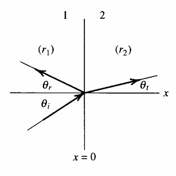
The incident wave is in the bottom left and forms an angle \theta_i with respect to the horizontal. Since the fluid boundary is vertical along x=0, this angle is formed parallel to the boundary normal and is called the incident angle. Like before, the wave is divided into a transmitted portion and reflected portion, each forming their own respective angles with the horizontal. Assume each fluid has an impedance z_1\neq z_2. Note that in Fig. 2, r_1 and r_2 denote impedances. We will stick to our z_1 and z_2 convention, however.
Constraints
Continuity of Pressure
Therefore, we see that the incident angle and reflected angle must be identical.
\boxed{\theta_i=\theta_r} \tag{25}
Additionally, we may consider the last two expressions to derive Snell’s Law between the incident and transmitted angles.
\boxed{\frac {\sin\theta_i}{c_1}=\frac {\sin\theta_t}{c_2}} \tag{26}
From this, it is clear to see that
\boxed{1+\underline R=\underline T} \tag{27}
Continuity of Normal Particle Velocities
Unlike the previous sections, where the total particle velocity must be the same across a boundary, an oblique incident only requires the normal particle velocity component be the same. Since particles may slip along the boundary, we have that u_x be equal on both sides for our choice of coordinate system in Fig. 2.
Transmission and Reflection Coefficients
Solving the system of equations above gives
\begin{aligned} &\boxed{ \mathrlap{\underline T=\frac{2z_2\sec\theta_t}{z_2\sec\theta_t+z_1\sec\theta_i}} \phantom{\underline R=\frac{z_2\sec\theta_t-z_1\sec\theta_i}{z_2\sec\theta_t+z_1\sec\theta_i}} }\\[8pt] &\boxed{ \underline R=\frac{z_2\sec\theta_t-z_1\sec\theta_i}{z_2\sec\theta_t+z_1\sec\theta_i} } \end{aligned} \tag{28}
Intensity Transmission and Reflection Coefficients
Special Cases
Case 1: c_1>c_2
If the sonic velocity in medium 2 is smaller than that of medium 1’s, such as the case of a wave propagating from water into air, Snell’s Law states
\theta_t=\arcsin\left(\frac {c_2}{c_1}\sin\theta_i\right)
If c_2<c_1, we must have that \theta_t<\theta_i. The transmitted wave will propagate in a direction closely parallel to the interface normal (i.e., almost horizontal in Fig. 2) as \theta_t will be small.
Case 2: c_1<c_2
If we reverse the situation, that is consider a wave propagating from air to water, we see that \theta_t>\theta_i from Eq. 26 and the transmitted wave will propagate almost parallel to the fluid boundary.
From Snell’s Law, we can see that there is indeed a limit to the value of \theta_t possible. If c_2\gg c_1 such that \frac {c_2}{c_1}\sin\theta_i>1, then no real value of \theta_t will satisfy Eq. 26.
\sin\theta_t=\frac {c_2}{c_1}\sin\theta_i
Evidently, there wil be a point where \frac {c_2}{c_1}\sin\theta_i=1 for a given value of c_2 relative to c_1. The value of \theta_i at that condition is called the critical angle and is often denoted as \theta_c instead of \theta_i.
\theta_c=\arcsin\left(\frac {c_1}{c_2}\right) \tag{29}
When \theta_i>\theta_c, there can be no real solution for \theta_t.
Case 3: \theta_i>\theta_c
To consider what happens when the incident angle exceeds the critical angle, we must investigate the behavior of \underline p_t and express \theta_t in terms of \theta_i.
The result is
\underline p(x, y, t)=\underline{\underline p}_te^{-k_2\sqrt{\left(\frac {c_2}{c_1}\right)^2\sin^2\theta_i-1}}e^{j(\omega t-k_2\frac {c_2}{c_1}y\sin\theta_i)}=\underline{\underline p}_te^{-\gamma x}e^{j(\omega t-k_2\frac {c_2}{c_1}y\sin\theta_i)}
Taking the real part of \underline p(x, y, t) to determine the physical pressure of the transmitted wave, we get
p_t(x, y, t)=\left|\underline{\underline p}_t\right|e^{-\gamma x}\cos\left(\omega t-k_2\frac {c_2}{c_1}y\sin\theta_i\right)=A(x)\cos\phi(y, t) \tag{30}
The amplitude in front of the exponential is only a function of x whereas the phase in the sinusoid is only a function of y and t (it is not a function of x). What this means is spatially, the wave has constant phase along each line of constant x, but its amplitude decreases as x increases. The wave has two characteristic traits: it propagates in y but decays in amplitude in x.
Such a wave, one that does not propagate through space but instead decays exponentially with distance, is called an evanescent wave. This kind of acoustic structure actually is not a wave, but is referred to as one based off terminology. For Eq. 30, we say the wave is evanescent in x and propagating in y.
Fluid-Solid Boundaries
Normal Incidence
We replace the solid with its normal specific acoustic impedance \underline z_m. The real part is the resistance r_m and the imaginary part is the reactance x_m.
\underline z_m=r_m+jx_m \tag{31}
From the definition of
Transmission and Reflection Coefficients
Replace all instances of z_2 in Eq. 8, which was a real quantity for fluid-fluid boundaries, with z_m in Eq. 31. For instance, the reflection and transmission coefficients are
\begin{aligned} &\boxed{ \mathrlap{\underline T=\frac{2\underline z_m}{z_1+\underline z_m}=\frac{2\underline z_m/z_1}{1+\underline z_m/z_1}} \phantom{\underline R=\frac{\underline z_m-z_1}{z_1+\underline z_m}=\frac{\underline z_m/z_1-1}{\underline z_m/z_1+1}} }\\[8pt] &\boxed{ \underline R=\frac{\underline z_m-z_1}{z_1+\underline z_m}=\frac{\underline z_m/z_1-1}{\underline z_m/z_1+1} } \end{aligned} \tag{32}
Intensity Transmission and Reflection Coefficients
We have once again that R_I=\left|\underline R\right|^2. Using Eq. 32, then
\begin{aligned} &\boxed{ \mathrlap{T_I=\frac{4r_mz_1}{(r_m+z_1)^2+x_m^2}} \phantom{R_I=\left[\frac{(r_m-z_1)^2+x_m^2}{(r_m+z_1)^2+x_m^2}\right]^2} }\\[8pt] &\boxed{ R_I=\left[\frac{(r_m-z_1)^2+x_m^2}{(r_m+z_1)^2+x_m^2}\right]^2 } \end{aligned} \tag{33}
The equation for T_I in Eq. 33 is also called the absorption coefficient and is denoted by \alpha_0. This quantity is unitless and represents the portion of the acoustic wave that is absorbed by the solid surface.
\boxed{\alpha_0=\frac {4r_mz_1}{(r_m+z_1)^2+x_m^2}} \tag{34}
Oblique Incidence
Though \underline p_i is a purely longitudinal wave, \underline p_t will likely have both longitudinal and shear components.
Anisotropic Solid
Isotropic Solid
If the solid properties vary uniformly regardless of direction, the solid is said to be isotropic. If we make the assumption that c_2\ll c_1, then Eq. 26 predicts \theta_t\simeq0^{\circ}. That is, the transmitted angle will be very small and \underline p_t will propagate nearly parallel in direction to the surface normal. For these cases, replace all instances of z_2\sec\theta_t with \underline z_m in Eq. 28. Therefore
\begin{aligned} &\boxed{ \mathrlap{\underline T=\frac{\underline z_m}{\underline z_m+z_1\sec\theta_i}} \phantom{\underline R=\frac{\underline z_m-z_1\sec\theta_i}{\underline z_m+z_1\sec\theta_i}} }\\[8pt] &\boxed{ \underline R=\frac{\underline z_m-z_1\sec\theta_i}{\underline z_m+z_1\sec\theta_i} } \end{aligned} \tag{35}