Introduction to Partial Differential Equations
Example 1 Consider the variable-form of the PDE where the wave speed a now depends on both position and time.
\begin{aligned} u_t+a(x, t)u_x & =0 \\ u(x, 0) & =u_0(x) \end{aligned} \tag{1}
Solution 1. Unlike the simple wave equation with constant a, the variable form will have nonlinear characteristic curves. Assume these curves can be described by (x(t), t) where x(t) is some unknown time-dependent function. Note here that we are using x as a function to describe the spatial coordinate of our characteristic curve, as well as the spatial coordinate of the entire PDE. We then proceed to define g(t) as
g(t)=u(x(t), t)
We want to investigate how g(t) behaves across t by taking the partial derivatives and relating to Eq. 1. By chain rule, g'(t) is
\frac {\mathrm dg}{\mathrm dt}=g'(t)=\frac {\partial u}{\partial x}\frac {\mathrm dx}{\mathrm dt}+\frac {\partial u}{\partial t}=u_x(x(t), t)x'(t)+u_t(x(t), t) \tag{2}
The goal here is to have Eq. 2 match the PDE in Eq. 1 such that the RHS is a known function of t. Comparing the two directly, we require
x'(t)=a(x(t), t) \tag{3}
If Eq. 3 is satisfied, then
g'(t)=a(x, t)u_x(x(t), t)+u_t(x(t), t)=0
In other words, under Eq. 3, g(t) is constant. For most problems we are given the form of a(x, t) as that is the coefficient of u_x. Thus, Eq. 3 becomes an ODE in t that may be solved to recover the characteristic curve of Eq. 1.
The equation of characteristics for this problem is
\left\{ \begin{aligned} x'(t) & =a(x, t) \\ x(0) & =x_0 \end{aligned} \right. \tag{4}
Once x(t) is known, then substitute t=0 to compute the initial spatial coordinate x_0. The coordinate (x_0, 0) is the position that the characteristic curve emanates from. With x_0 and therefore, u_0(x_0) known, then u(x, t)=u_0(x_0) since g'(t)=0.
Now let’s look at a specific example to illustrate how characteristic curves allow us to evaluate a PDE analytically.
Example 2 Consider the nonlinear PDE below. This is a special case of Eq. 1 with a(x, t)=x.
\begin{aligned} u_t+xu_x & =0 \\ u(x, 0) & =\begin{cases}1 & \qquad 0\leq x\leq 1 \\0 & \qquad\mathrm{otherwise}\end{cases} \end{aligned} \tag{5}
Solution 2. The initial condition is given as a piecewise constant function that is not continuous and differentiable at all. However, we can still solve this since we allow discontinuous solutions for hyperbolic functions. From Eq. 4, we have
\left\{ \begin{aligned} x'(t) & =x \\ x(0) & =x_0 \end{aligned} \right.
This is a simple ODE that can be solved by separation of variables to obtain x(t)=x_0e^t. The characteristic curves for Eq. 5 are therefore exponential, following e^t that originate from (x_0, 0). For a given (x, t) whose characteristic curve originates from (x_0, 0), then
x_0=xe^{-t}
Therefore, u(x, t) can be computed as
u(x, t)=u(x_0, 0)=u_0(xe^{-t})
Boundary Conditions
Boundary Values
Let’s consider the 1D transport problem, u_t+au_x=0, restricted to a finite interval. Without loss of generality, we may assume the interval to be 0\leq x\leq 1. Depending on the value of the wave speed a, the characteristic curves may be lines of positive or negative slope as shown below.
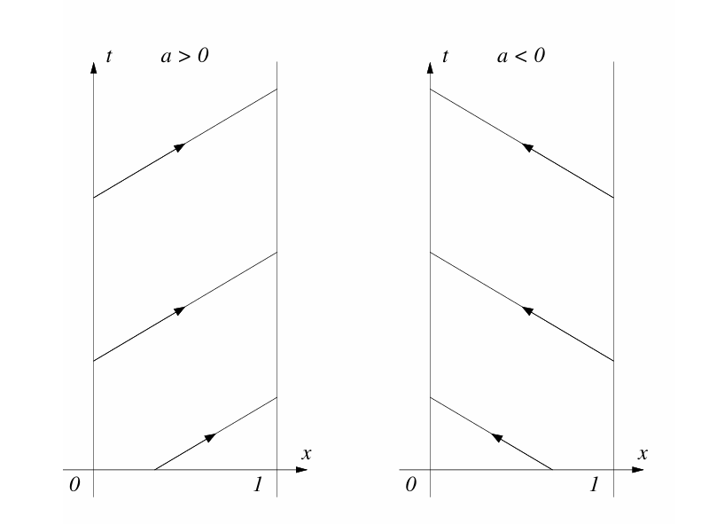
We have shown that for the case of u_t+au_x=0, the solution u(x, t) is constant along each characteristic x-at.
If a>0, so the characteristics propagate towards the right, then the solution should be specified on the boundary at x=0 in addition to the initial data at t=0.
Remark 1. No data can be specified at the other boundary, x=1 in this case, otherwise you will have an overconstrained equation.
Specifying the solution at x=1, in addition to the initial data at t=0, is also valid as u(x, t) may be solved traveling back towards x=0 along the characteristic. But generally, it is more likely that the solution at the x=0 boundary be specified.
If a<0, the solution should be specified at the boundary x=1 in addition to the initial data at t=0. The solution can then be solved along each characteristic to achieve the solution at the x=0 boundary.
Periodic Problems
The second type of boundary we may encounter are periodic boundaries. To illustrate, we consider the 1D transport equation on the restricted interval 0\leq x\leq 1. Instead of specifying the value directly at the boundaries, we relate them to each other \forall t\geq0.
u(0, t)=u(1, t)
Periodic boundary conditions are equivalent to a PDE being specified on the entire real line -\infty<x<\infty satisfying u(x+1, t)=u(x, t) for all x and t.
Finite Difference Schemes
For finite difference schemes (FDS), the idea is very simple: instead of storing all values of u(x, t) across all time and space, store discrete values of u in a grid and compute the derivatives using its definition. Consider a grid on the x-t plane. Presume that the grid is uniform in space and time as shown below.
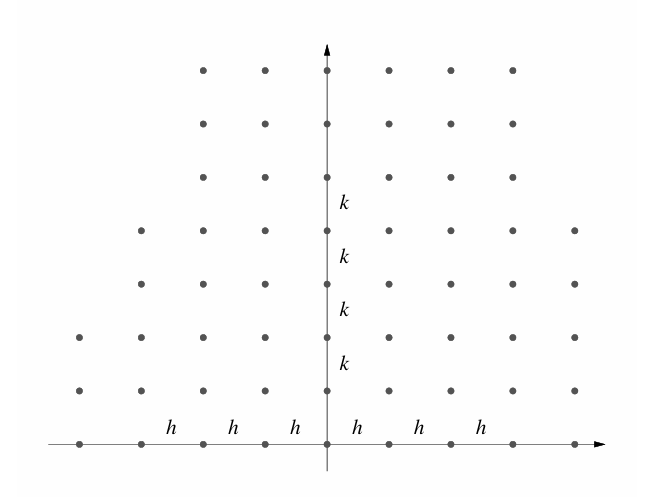
The distance between two adjacent grid points spatially is denoted by h=\Delta x. Similarly, the distance between two adjacent points along the time axis is denoted by k=\Delta t.
The grid points are denoted as
(x_m, t_n)=(m\Delta x, n\Delta t)=(mh, nk)
Let v be a function defined on the grid. Then we define v_m^n as the value of v at the grid point (x_m, t_n).
If u(x, t) is a function defined for continuously varying (x, t), such as the ground-truth solution to the PDE, then we also use u_^n to denote the value of u at the grid point (x_m, t_n). In other words, u_m^n=u(x_m, t_n).
The set of points (x_m, t_n) for a fixed value of n is called the grid level n. For example, grid level 2 refers to the collection of points along the grid that make up (x_m, t_2) (e.g., the third row of grid points in the discretized x-t plane).
We are interested in grids with small $$.
Definition 1 To derive a finite difference scheme from its continuous functional counterpart, replace all derivatives with their finite difference representations. For example, if our PDE contains the partial derivative \frac {\partial u}{\partial t}, we may approximate this on a discrete set of points using
\begin{aligned} \frac {\partial u}{\partial t}(x_m, t_n)=\lim\limits_{k\to0}\frac {u(x_m, t_n+k)-u(x_m, t_n)}k & \approx\frac {u(x_m, t_n+k)-u(x_m,t_n)}k\\ & \approx\frac {u(x_m, t_n+k)-u(x_m, t_n-k)}{2k} \end{aligned}
Finite differences become more accurate as k\to0 per their limit definitions.
Consider the 1D convection equation u_t+au_x=0. We have the following five finite difference schemes to approximate and numerically solve this equation.
Forward-Time, Forward-Space (FTFS) scheme
\frac {v_m^{n+1}-v_m^n}k+a\frac {v_{m+1}^n-v_m^n}h=0 \tag{6}
We use forward difference schemes to compute both the time and spatial derivatives. For each direction, we step forward in time or space and subtract the current point v_m^n to compute the derivative. For this reason, it is called the forward time and forward space scheme.
Forward-Time, Backwards-Space (FTBS) Scheme
\frac {v_m^{n+1}-v_m^n}k+a\frac {v_m^n-v_{m-1}^n}h=0 \tag{7}
The time derivative is identical to Eq. 6 as we are stepping forward in time and moving up a grid level when computing v_m^{n+1}. However, the spatial term is different: instead of stepping forward to calculate the spatial derivative, we are actually stepping backwards. For this reason, this is called the FTBS scheme.
Forward-Time, Central-Space (FTCS) Scheme
\frac {v_m^{n+1}-v_m^n}k+a\frac {v_{m+1}^n-v_{m-1}^n}{2h}=0 \tag{8}
Leapfrog Scheme
\frac {v_m^{n+1}-v_m^{n-1}}{2k}+a\frac {v_{m-1}^n+v_{m+1}^n}{2h}=0 \tag{9}
We use central difference schemes for computing both the time and space derivatives. Unlike the previous schemes, we do not use v_m^n in this scheme.
Lax-Friedrichs Scheme
\frac {v_m^{n+1}-\frac 12\left(v_{m-1}^n+v_{m+1}^n\right)}k+a\frac {v_{m+1}^n-v_{m-1}^n}{2h}=0 \tag{10}
Like Eq. 9, we do not use v_m^n when computing v_m^{n+1}. The spatial derivative is computed with central difference, much like Eq. 8. However, the temporal derivative is computed by subtracting a “predicted” value of v_m^n from v_m^{n+1}. Instead of directly using v_m^n, we compute it from its neighbors, v_{m-1}^n and v_{m+1}^n.
Remark 2. Note that the schemes presented in Eq. 6 through Eq. 10 are explicit and can be written by expressing v_m^{n+1} as a linear combination of values of v at grid levels n and n-1. For example, with Eq. 6, solve for v_m^{n+1} to get
v_m^{n+1}=(1+a\lambda)v_m^n-a\lambda v_{m+1}^n
where \lambda=\frac kh=\frac {\Delta t}{\Delta x}. The variable \lambda is a very important quantity that will play a significant role when analyzing these difference schemes.
Definition 2 Schemes that involve v at only two grid levels, n+1 and n, are called one-step schemes. Given initial condition data v_m^0, subsequent grid levels v_m^1, v_m^2, etc. are computed one step at a time.
Schemes that involve v at more than two grid levels are called multi-step schemes. They require knowing how the grid function behaves at multiple grid levels to compute the next one. For example, the Leapfrog scheme given by Eq. 9 requires knowing the values of v at grid levels n and n-1 to compute v_m^{n+1}. That is, to compute v_m^2, we must know v_m^0 and v_m^1.
Generally, only initial data at t=0 is known for a given problem. To apply multi-step schemes, we require applying one-step schemes to determine the behavior of v_m^1 and above grid levels, before we may apply the multi-step scheme itself.
Example 3 Consider the 1D transport equation with a=1 for -2\leq x\leq 3 and t\geq0.
\begin{aligned} u_t+u_x & =0 \\ \\ u_0(x) & =\begin{cases}1-|x| & \qquad|x|\leq1 \\0 & \qquad|x|>1\end{cases} \\ \\ u(-2, t) & =0 \end{aligned}
Solution 3. This problem is well-posed since there is an initial condition at t=0 and a boundary value specified at x=-2 for constant transport. If we implemented a finite difference scheme to numerically solve this problem, we see drastically different behaviors depending on the value of \lambda used. For Example 3, we apply Eq. 10 with different values of \lambda.
With \lambda=0.8 and h=0.1, the numerical solution is shown below.
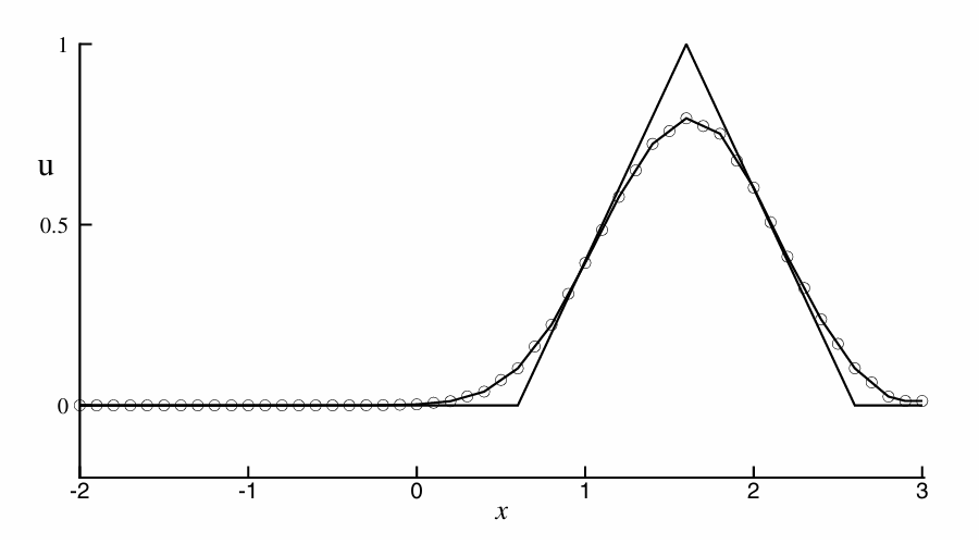
A solution of the Lax-Friedrichs scheme with \lambda=0.8 With \lambda=1.6 and h=0.1, the numerical solution is unstable.
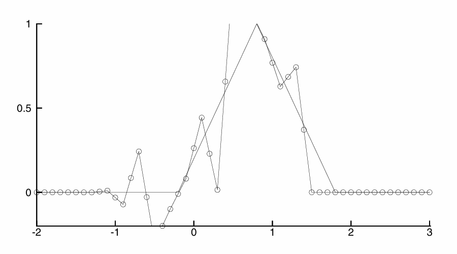
A solution of the Lax-Friedrichs scheme with \lambda=1.6
Convergence and Consistency
For a given scheme used to approximate the solution to a PDE, convergence simply reflects the ability of the numerically computed solution to become closer and closer towards the ground-truth solution as (h,k)\to(0, 0). That is, as the computational grid is refined, the numerical solution become the analytical solution.
We have seen previously with the Lax-Friedrichs scheme that having (h,k)\to(0, 0) is not a sufficient condition for guaranteeing convergence; the path taken by (h,k) also matters.
Consider a linear PDE of the form
P(\partial_t, \partial_x)u=f(x, t) \tag{11}
The only requirement we have is that Eq. 11 be first-order with respect to time. The differential equation itself may contain higher order spatial derivatives (e.g., u_{xx} or u_{tx}). Examples of valid PDEs under this requirement include
\begin{aligned} u_t-bu_{xx}+au_x & =0 \\ u_t+cu_{tx}+au_x & =f(x, t) \end{aligned}
For each PDE above, the highest order for the time derivative is first order (the u_{tx} term does not count as it is also differentiated with respect to x). And lastly, we assume the problem given by Eq. 11 is well-posed, where given an initial condition u(x_0)=u_0(x), there is a unique solution to Eq. 11.
Definition 3 (Convergent Scheme) A one-step finite difference scheme approximating a PDE is called a convergent scheme if for any solution u(x, t) that satisfies the PDE and solution v_m^n to the finite difference scheme, v_m^n\to u(x, t) as (mh, nk)\to(x, t) and (h,k)\to0. We, of course, require that v_m^0 converges to u_0(x) as mh\to x.
Proving that a finite difference scheme is convergent directly is difficult. However, there are two related concepts that are easy to verify. They are consistency and stability. Together, these conditions are sufficient to determine whether a finite difference scheme is convergent, as we will see later on.
Definition 4 (Consistency) Given a PDE of the form P(\partial_t, \partial_x)u=f and a finite difference scheme P_{h,k}v=f, we say that the finite difference scheme is consistent with the PDE if for any smooth function \phi(x, t), we have as (h,k)\to0
P\phi-P_{h,k}\phi\to0 \tag{12}
The convergence in this case being the pointwise convergence at each (x, t).
Remark 3. For some finite difference scheme, we need to restrict the manner in which (h,k)\to0 for the scheme to be consistent. To illustrate this, if we imagine (h,k) as two arbitrarily positive numbers in the positive h-k plane, (h,k)\to0 describes some sequence or path taken towards the origin.
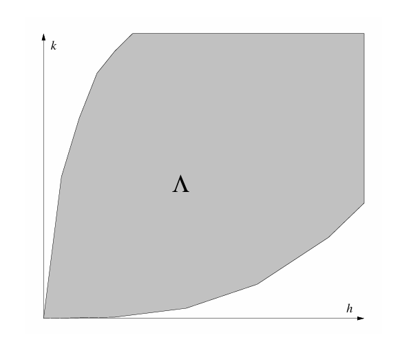
Certain finite difference schemes may be inconsistent for arbitrarily chosen values of (h,k). However, if we restrict our choice to be within a region of stability defined by \Lambda, the scheme may become consistent.
We also require \phi(x, t) to be a smooth function, meaning it is sufficiently differentiable for the context of the problem.
Remark 4. The differential operator P_{h,k} when applied to \phi(x, t) does not need to be restricted to the grid. For example, with the forward difference scheme, we have
P_{h,k}\phi(x, t)=\frac {\phi(x+h, t)-\phi(x, t)}h
Define the differential operator as P=\partial_t+a\partial_x. When applied to the arbitrary smooth function \phi(x, t), then
P\phi=\phi_t+a\phi_x \tag{13}
The FTFS scheme is
\left(P_{h,k}\phi\right)_m^n=\frac {\phi_m^{n+1}-\phi_m^n}k+\frac {\phi_{m+1}^n-\phi_m^n}h \tag{14}
We want to show that as (h,k)\to0, then Eq. 14 for any point becomes Eq. 13. To accomplish this, we take the Taylor expansion of each term in x and t.
\begin{aligned} \phi_m^{n+1} & =\phi_m^n+k\phi_t+\frac 12k^2\phi_{tt}+\mathcal O(k^3) \\ \phi_{m+1}^n & =\phi_m^n+h\phi_x+\frac 12h^2\phi_{xx}+\mathcal O(h^3) \end{aligned} \tag{15}
In this notation, the derivatives are understood to be evaluated at the point of interest, (mh, nk). Substitute the expansions in Eq. 15 into Eq. 14 and simplify.
\left(P_{h,k}\phi\right)_m^n=\phi_t+a\phi_x+\frac 12k\phi_{tt}+\frac 12ah\phi_{xx}+\mathcal O(k^2)+\mathcal O(h^2) \tag{16}
This operator when applied onto \phi is not limited to a certain set of points. That is, we may choose an arbitrary (x, t) to apply Eq. 16 on. We can show that the difference between Eq. 13 and Eq. 16 becomes zero as (h,k)\to0.
P_{h,k}\phi-P\phi=\frac 12k\phi_{tt}+\frac 12ah\phi_{xx}+\mathcal O(k^2)+\mathcal O(h^2)\to0
Maintain the same definition for the differential operator as P=\partial_t+a\partial_x. The differential operator for the Lax-Friedrichs scheme is
P_{h,k}\phi=\frac {\phi_m^{n+1}-\frac 12\left(\phi_{m+1}^n+\phi_{m-1}^n\right)}k+a\frac {\phi_{m+1}^n-\phi_{m-1}^n}{2h}
Applying a Taylor expansion to \phi_{m\pm1}^n and \phi_m^{n+1} and substituting, we get
P_{h,k}\phi=\phi_t+a\phi_x+\frac 12k\phi_{tt}-\frac 12\frac {h^2}k\phi_{xx}+\frac 16ah^2\phi_{xxx}+\mathcal O\left(h^4+\frac {h^4}k+k^2\right) \tag{17}
The form of Eq. 17 is very similar to that given in Eq. 16. However, the rate at which h\to0 and k\to0 now matter. If k\to0 at a much faster rate than h\to0, then the \frac {h^2}k term will blow up. Therefore, P_{h,k}\phi-P\phi\to0 as (h,k)\to0 as long as \frac {h^2}k\to0.
Recall that in Example 3, we observed how the value of \lambda affects the behavior of the numerical solution when using Lax-Friedrichs. In fact, choosing too large of a \lambda resulted in the numerical solution blowing up. From the consistency proof here, we can conclude that this observed instability is not caused by Eq. 10 being inconsistent. The reason for this is if we maintain a constant \lambda=\frac kh, as was done in the example, then \frac {h^2k}=\frac h{\lambda}\to0 as (h,k)\to0 so the scheme is consistent. We will eventually see that the issue arises when proving stability.
Proving consistency is not a sufficient condition for proving convergence. We can show that a consistent scheme exists that is not (or even never) convergent! For our example, we consider the FTFS scheme, Eq. 6, applied to u_t+u_x=0.
Consider the 1D convection equation with unit wave speed subject to the initial condition
u_0(x)=\begin{cases}1 & \qquad-1\leq x\leq0 \\0 & \qquad\mathrm{otherwise}\end{cases}
The analytical solution to the PDE is given in the image below. The solution at grid point (x_m,t_n) is given by shifting u_0 to the right by t. The solid diagonal lines in Fig. 2 denote the characteristic lines where u(x, t) becomes nonzero. Outside of this “band”, u(x,t)=0.
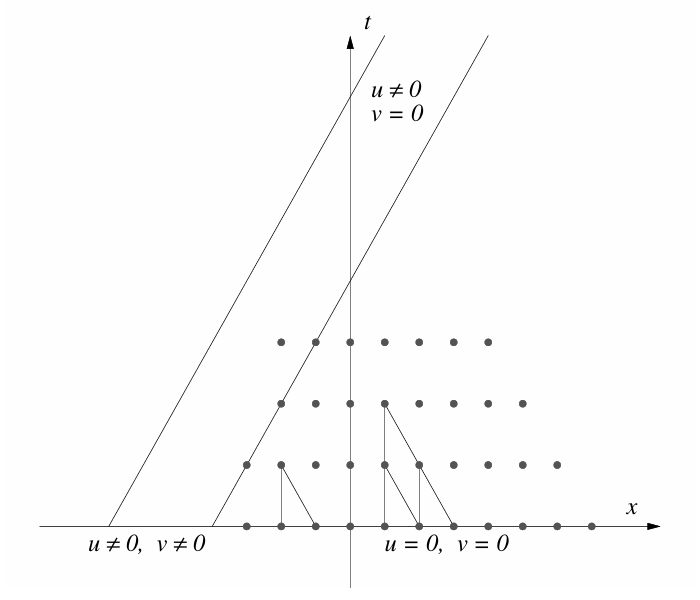
For the difference scheme, take the initial data to be
v_m^0=\begin{cases}1 & \qquad-1\leq mh\leq 0 \\0 & \qquad\mathrm{otherwise}\end{cases}
From Eq. 6, we can see that v_m^{n+1} is dependent only on v_m^n and v_{m+1}^n. Therefore, Eq. 6 will predict v_m^{n+1}=0 for x\geq0 as v_m^n=0 and v_{m+1}^n=0 in this region. The numerical solution disagrees with the solution presented in Fig. 2, as it does not predict the sloped characteristic curves that delineate where u(x,t)\neq0.
As a result, we may conclude Eq. 6 is nonconvergent. Yet, we have successfully shown that Eq. 6 is consistent. Therefore, consistency alone is not a sufficient condition for determining convergence.
Stability
When performing stability analysis, we only need to consider the homogeneous form of the PDE. That is, if the general form of the differential equation is Pu=f, we only need to consider Pu=0 in our stability analysis.
A stability region \Lambda is any subset of \mathbb R_{>0}^2 that has the origin (0, 0) as an accumulation point.
Graphically, in Fig. 1, we may imagine a region in the first quadrant of the h-k plane. All values of (h, k) in this region are stable, and this region called \Lambda includes the origin. There is some sequence or path where (h, k)\to0 and the scheme remains stable.
A finite difference scheme P_{h,k}v_m^n=0 for a PDE that is first-order in time is stable in a stability region \Lambda if there is an integer J such that for any positive time T, there is a constant C_T>0 such that
h\sum\limits_{m=-\infty}^{\infty}\left|v_m^n\right|^2\leq C_Th\sum\limits_{j=0}^J\sum\limits_{m=-\infty}^{\infty}\left|v_m^j\right|^2 \tag{18}
for 0\leq nk\leq T with (h,k)\in\Lambda.
Remarks:
If \left(\omega_m\right)_{m=-\infty}^{\infty} is a function on a spatial grid of h, then define the L2 norm of the grid function \omega as
\lVert\omega\rVert_h=\left(h\sum\limits_{m=-\infty}^{\infty}\left|\omega_n\right|^2\right)^{1/2} \tag{19}
The RHS of Eq. 19 looks very similar to a Riemann sum. Indeed, the integral form where the infinite sum is replaced with an integral is the continuous L2 norm definition. Therefore, Eq. 19 defines a discrete L2 norm definition that attempts to approximate the continuous L2 norm of a function.
The stability definition in Eq. 18 is fundamentally a relationship between the discrete L2 norms of v.
With this notation, we can rewrite Eq. 18 as
\lVert v^n\rVert_h^2\leq C_T\sum\limits_{j=0}^J\left\lVert v^j\right\rVert_h^2
This version of stability says that the L2 norm of v at a future time is bounded or controlled by the L2 norms at previous time. This is also equivalent to
\lVert v^n\rVert_h\leq C_T^*\sum\limits_{j=0}^J\left\lVert v^j\right\rVert_h \tag{20}
Eq. 20 effectively says that the h-norm of the solution at any time t\leq T has an upper limit on its growth; it cannot grow unbounded.
The purpose of J is to accommodate the definition for multi-step schemes. For one-step schemes, J=0 and the RHS of Eq. 20 reduces down to
\lVert v^n\rVert_h\leq C_T^*\left\lVert v^0\right\rVert_h
The growth at the nth time level is bounded by the growth at the initial time. We must choose specific (h,k) such that Eq. 20 does not blow up.
To illustrate the essence of stability, we apply Note 4 to show how Eq. 6 is unstable and therefore, cannot be convergent.
Instead of deriving the stability condition valid only for Eq. 6, we may consider the general form of the FTFS scheme and derive a broader stability requirement. Consider the general form of the FTFS scheme below.
v_m^{n+1}=\alpha v_m^n+\beta v_{m+1}^n \tag{21}
The FTFS scheme for solving u_t+u_x=0 is a special case where \alpha=1+a\lambda and \beta=-a\lambda. We can show that Eq. 21 is stable if and only if
|\alpha|+|\beta|\leq1 \tag{22}
To prove this, we take the LHS of Eq. 18 and manipulate the LHS to be in terms of v_m^0, the initial condition. Substitute the definition of the scheme and apply the triangle inequality theorem.
\begin{aligned} \sum\limits_{m=-\infty}^{\infty}\left|v_m^{n+1}\right|^2 & =\sum\limits_{m=-\infty}^{\infty}\left|\alpha v_m^n+\beta v_{m+1}^n\right|^2 \\ & =\sum\limits_{m=-\infty}^{\infty}\alpha^2\left|v_m^n\right|^2+2\left|\alpha\right|\left|\beta\right|\left|v_m^n\right|\left|v_{m+1}^n\right|+\beta^2\left|v_{m+1}^n\right|^2 \\ & \leq\sum\limits_{m=-\infty}^{\infty}\alpha^2\left|v_m^n\right|^2+\left|\alpha\right|\left|\beta\right|\left(\left|v_m^n\right|^2+\left|v_{m+1}^n\right|^2\right)+\beta^2\left|v_{m+1}^n\right|^2 \\ & =\sum\sum\limits_{m=-\infty}^{\infty}\alpha^2\left|v_m^n\right|^2+\left|\alpha\beta\right|\left|v_m^n\right|^2+\sum\limits_{m=-\infty}^{\infty}\left|\alpha\beta\right|\left|v_{m+1}^n\right|^2+\beta^2\left|v_{m+1}^n\right|^2 \end{aligned}
Note that in the penultimate equation, we use the fact that 2xy\leq x^2+y^2. The second summation can be re-indexed such that v_{m+1}^n\to v_m^n. The bounds of m remain the same since -\infty<m<\infty. Therefore, we get
\sum\limits_{m=-\infty}^{\infty}\left|v_m^{n+1}\right|^2=\sum\limits_{m=-\infty}^{\infty}\left(\left|\alpha\right|^2+2\left|\alpha\right|\left|\beta\right|+\left|\beta\right|^2\right)\left|v_m^n\right|^2=\left(\left|\alpha\right|+\left|\beta\right|\right)^2\sum\limits_{m=-\infty}^{\infty}\left|v_m^n\right|^2
We have managed to relate the L2 norm of v at grid level n+1 to the L2 norm of v at grid level n. We may repeat this same process on \left|v_m^n\right|^2 to relate it to the L2 norm of v at grid level n-1. By induction, we can show that the equation above can be related to the initial L2 norm.
\sum\limits_{m=-\infty}^{\infty}\left|v_m^n\right|^2\leq\left(\left|\alpha\right|+\left|\beta\right|\right)^{2n}\sum\limits_{m=-\infty}^{\infty}\left|v_m^0\right|^2\leq\sum\limits_{m=-\infty}^{\infty}\left|v_m^0\right|^2 \tag{23}
Therefore, the stability condition is
\left|\alpha\right|+\left|\beta\right|\leq C_T=1
We may relate the concept of stability to the well-posedness of a PDE in a similar form as Eq. 18.
The initial value problem for a homogeneous PDE that is first-order in time, Pu=0, is well-posed if for any T\geq0, there exists a constant C_T such that any solution u(x, t) satisfies
\int_{-\infty}^{\infty}\left|u(x, t)\right|^2\,\mathrm dx\leq C_T\int_{-\infty}^{\infty}\left|u(x, 0)\right|^2\,\mathrm dx \tag{24}
for 0\leq t\leq T.
Remark: The numerical speed of propagation for a scheme of the form v_m^{n+1}=\alpha v_{m-1}^n+\beta v_m^n+\gamma v_{m+1}^n is \frac hk=\frac 1{\lambda}. For such a scheme to be stable, it is necessary that the numerical speed exceed the real speed of the PDE.
\frac 1{\lambda}\geq|a|